Sundar B. N.
Assistant Professor
Least Square Method
Fitting a Linear Trend Equation
Yearly Sales
Trend Values
Years From 2010 to 2017
Least Square Method
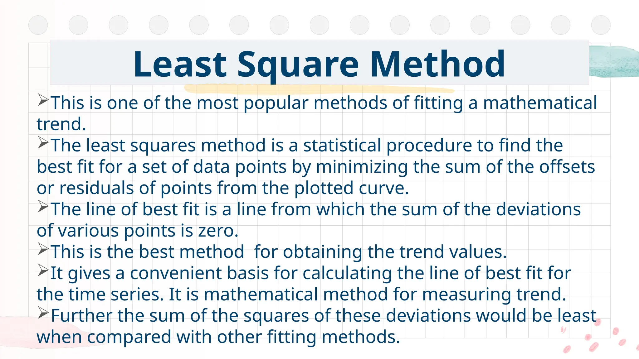
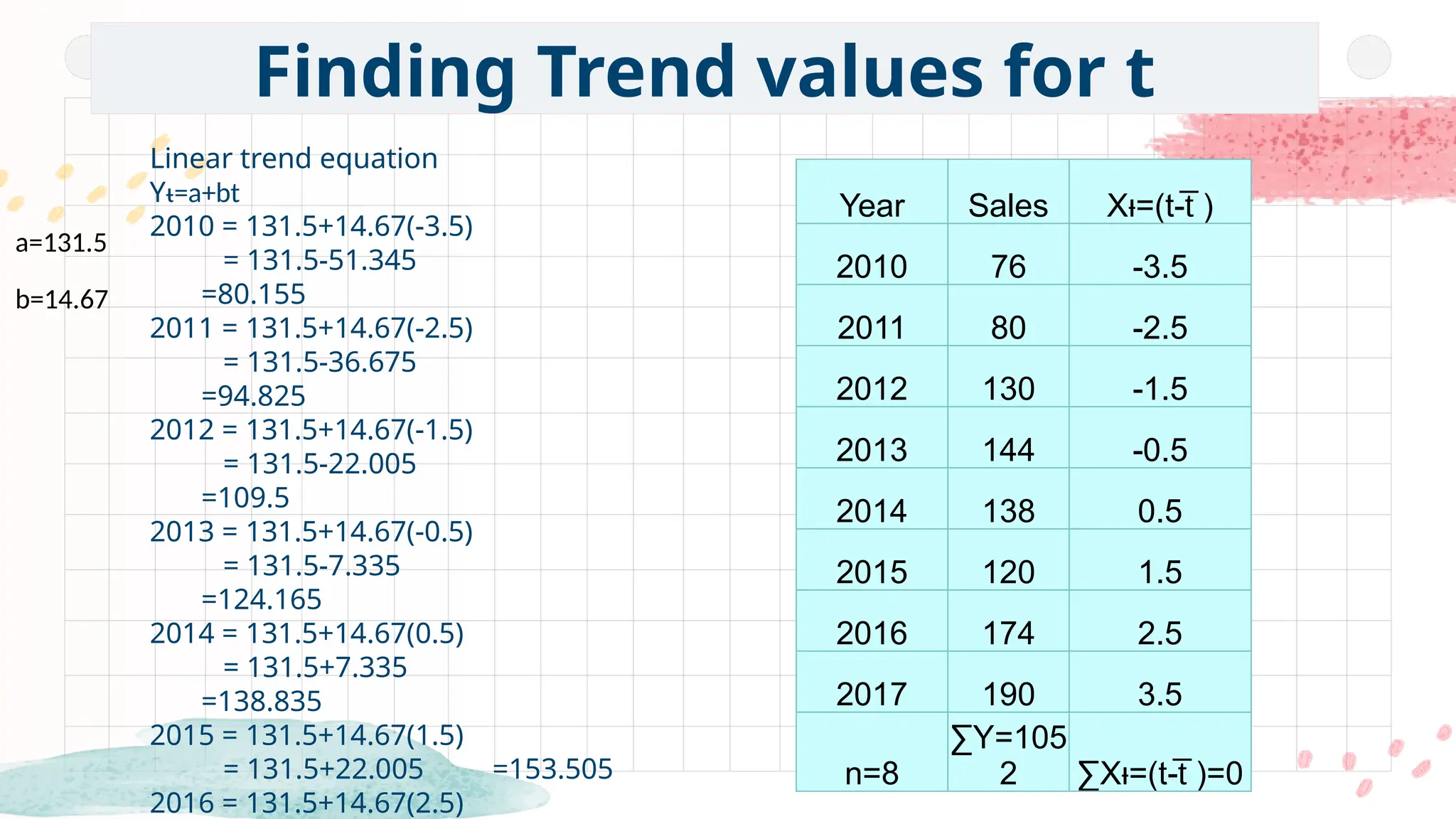
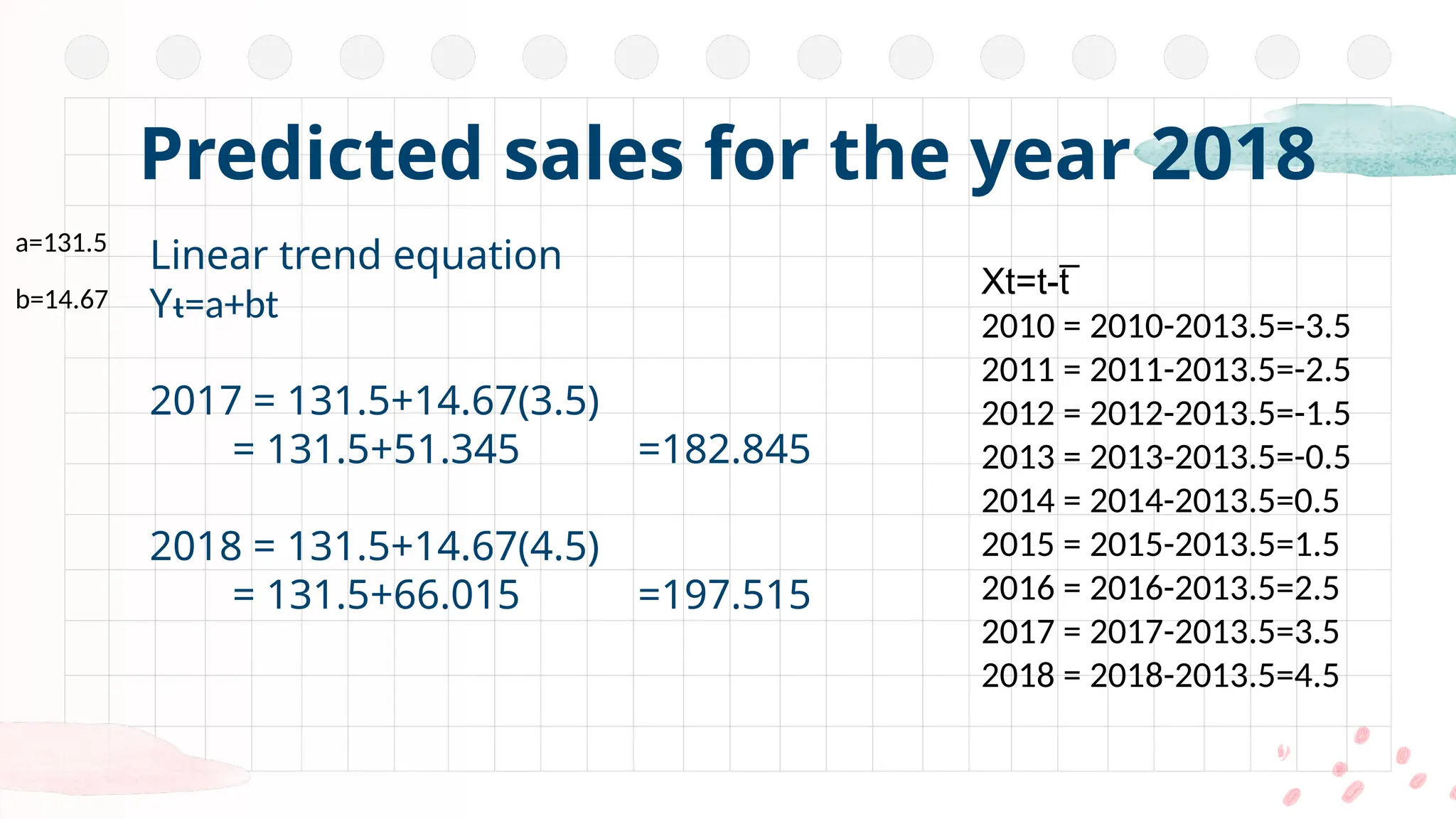
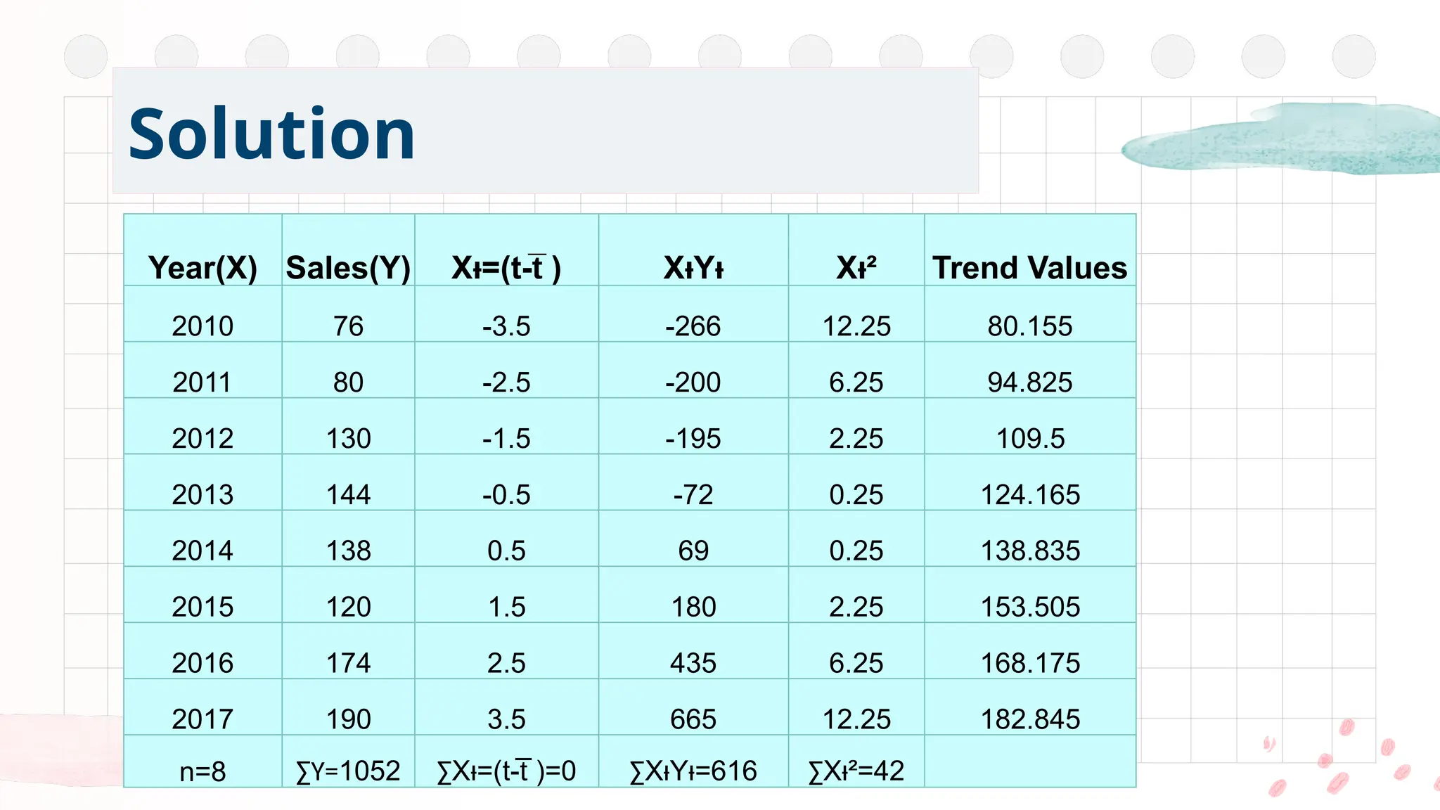
This is one of the most popular methods of fitting a mathematical
trend.
The least squares method is a statistical procedure to find the
best fit for a set of data points by minimizing the sum of the offsets
or residuals of points from the plotted curve.
The line of best fit is a line from which the sum of the deviations
of various points is zero.
This is the best method for obtaining the trend values.
It gives a convenient basis for calculating the line of best fit for
the time series. It is mathematical method for measuring trend.
Further the sum of the squares of these deviations would be least
when compared with other fitting methods.
Linear trend equation
Yᵼ=a+bt
Normal Equation for obtaining the values of a and b are
a = ∑Y/n
b = ∑XY/∑X²
t̅= ∑t/n
Formula
Fit a straight line trend by the method of least squares to the
following data. Assuming the same rate of change continues
what would be the predicted sales for the year 2018?
Calculate trend values from 2010 to 2017.
Problem
Year 2010 2011 2012 2013 2014 2015 2016 2017
Sales(Rs. In lakhs) 76 80 130 144 138 120 174 190
t̅= ∑t/n
=16108/8 t̅ =2013.5
Xt=t-t̅̅
2010 = 2010-2013.5=-3.5
2011 = 2011-2013.5=-2.5
2012 = 2012-2013.5=-1.5
2013 = 2013-2013.5=-0.5
2014 = 2014-2013.5=0.5
2015 = 2015-2013.5=1.5
2016 = 2016-2013.5=2.5
2017 = 2017-2013.5=3.5
2018 = 2018-2013.5=4.5
Solution - t̅= ∑t/n
Year Sales X =(t- )
ᵼ t̅
2010 76 -3.5
2011 80 -2.5
2012 130 -1.5
2013 144 -0.5
2014 138 0.5
2015 120 1.5
2016 174 2.5
2017 190 3.5
n=8
∑Y=10
52
∑X =(t-
ᵼ
)=0
t̅
Year
2010
2011
2012
2013
2014
2015
2016
2017
16108
Find XY and X²
Year(X) Sales(Y) X =(t- )
ᵼ t̅ X Y
ᵼ ᵼ X ²
ᵼ
2010 76 -3.5 -266 12.25
2011 80 -2.5 -200 6.25
2012 130 -1.5 -195 2.25
2013 144 -0.5 -72 0.25
2014 138 0.5 69 0.25
2015 120 1.5 180 2.25
2016 174 2.5 435 6.25
2017 190 3.5 665 12.25
n=8 ∑Y=1052 ∑X =(t- )=0
ᵼ t̅ ∑X Y =616
ᵼ ᵼ ∑X ²=42
ᵼ
Normal Equation for obtaining
the values of a and b are
a = ∑Y/n
=1052/8
a=131.5
b = ∑XY/∑X²
=616/42
b=14.67
Applying to Normal Equation
Year(X)
Sales(
Y) X =(t- )
ᵼ t̅ X Y
ᵼ ᵼ X ²
ᵼ
2010 76 -3.5 -266 12.25
2011 80 -2.5 -200 6.25
2012 130 -1.5 -195 2.25
2013 144 -0.5 -72 0.25
2014 138 0.5 69 0.25
2015 120 1.5 180 2.25
2016 174 2.5 435 6.25
2017 190 3.5 665 12.25
n=8 ∑Y=1052 ∑X =(t- )=0
ᵼ t̅ ∑X Y =616
ᵼ ᵼ ∑X ²=42
ᵼ
Linear trend equation
Yᵼ=a+bt
2010 = 131.5+14.67(-3.5)
= 131.5-51.345
=80.155
2011 = 131.5+14.67(-2.5)
= 131.5-36.675
=94.825
2012 = 131.5+14.67(-1.5)
= 131.5-22.005
=109.5
2013 = 131.5+14.67(-0.5)
= 131.5-7.335
=124.165
2014 = 131.5+14.67(0.5)
= 131.5+7.335
=138.835
2015 = 131.5+14.67(1.5)
= 131.5+22.005 =153.505
2016 = 131.5+14.67(2.5)
Finding Trend values for t
a=131.5
b=14.67
Year Sales X =(t- )
ᵼ t̅
2010 76 -3.5
2011 80 -2.5
2012 130 -1.5
2013 144 -0.5
2014 138 0.5
2015 120 1.5
2016 174 2.5
2017 190 3.5
n=8
∑Y=105
2 ∑X =(t- )=0
ᵼ t̅
Linear trend equation
Yᵼ=a+bt
2017 = 131.5+14.67(3.5)
= 131.5+51.345 =182.845
2018 = 131.5+14.67(4.5)
= 131.5+66.015 =197.515
Predicted sales for the year 2018
a=131.5
b=14.67
Xt=t-t̅̅
2010 = 2010-2013.5=-3.5
2011 = 2011-2013.5=-2.5
2012 = 2012-2013.5=-1.5
2013 = 2013-2013.5=-0.5
2014 = 2014-2013.5=0.5
2015 = 2015-2013.5=1.5
2016 = 2016-2013.5=2.5
2017 = 2017-2013.5=3.5
2018 = 2018-2013.5=4.5
Solution
Year(X) Sales(Y) X =(t- )
ᵼ t̅ X Y
ᵼ ᵼ X ²
ᵼ Trend Values
2010 76 -3.5 -266 12.25 80.155
2011 80 -2.5 -200 6.25 94.825
2012 130 -1.5 -195 2.25 109.5
2013 144 -0.5 -72 0.25 124.165
2014 138 0.5 69 0.25 138.835
2015 120 1.5 180 2.25 153.505
2016 174 2.5 435 6.25 168.175
2017 190 3.5 665 12.25 182.845
n=8 ∑Y=1052 ∑X =(t- )=0
ᵼ t̅ ∑X Y =616
ᵼ ᵼ ∑X ²=42
ᵼ
Computed trend line for the data of
Sales
Yearly Sales
Trend Values
Years From 2010 to 2017
Year
Yearly
Sales
Trend
Values
2010 76 80.155
2011 80 94.825
2012 130 109.5
2013 144 124.165
2014 138 138.835
2015 120 153.505
2016 174 168.175
2017 190 182.845
1. Given the mathematical form of the trend to be fitted, the least
squares method is an objective method.
2. Unlike the moving average method, it is possible to compute trend
values for all the periods and predict the value for a period lying
outside the observed data.
3. The results of the method of least squares are most satisfactory
because the fitted trend satisfies the two most important properties,
i.e. (1) (Y0 - Yt ) = 0 and (2) (Y0 - Yt )2 is minimum. Here Y0 denotes
∑ ∑
the observed values and Yt denotes the calculated trend value.
The first property implies that the position of fitted trend equation is such
that the sum of deviations of observations above and below this equal
to zero. The second property implies that the sums of squares of
deviations of observations, about the trend equations, are minimum.
Merits of Least Square Method
1. As compared with the moving average method, it is cumbersome
method.
2. It is not flexible like the moving average method. If some
observations are added, then the entire calculations are to be done
once again.
3. It can predict or estimate values only in the immediate future or the
past.
4. The computation of trend values, on the basis of this method,
doesn’t take into account the other components of a time series and
hence not reliable.
5. Since the choice of a particular trend is arbitrary, the method is not,
strictly, objective.
6. This method cannot be used to fit growth curves, the pattern
Demerits of Least Square
Method
 Bhardwaj, R. S. (2009). Business Statistics.
Excel Books India.
 Shukla, G. K.; Trivedi, Manish (2017). “Unit-13
Trend Component Analysis. IGNOU
Reference

Time Series Analysis - Least Square Method Fitting a Linear Trend Equation

  • 1.
    Sundar B. N. AssistantProfessor Least Square Method Fitting a Linear Trend Equation Yearly Sales Trend Values Years From 2010 to 2017
  • 2.
    Least Square Method Thisis one of the most popular methods of fitting a mathematical trend. The least squares method is a statistical procedure to find the best fit for a set of data points by minimizing the sum of the offsets or residuals of points from the plotted curve. The line of best fit is a line from which the sum of the deviations of various points is zero. This is the best method for obtaining the trend values. It gives a convenient basis for calculating the line of best fit for the time series. It is mathematical method for measuring trend. Further the sum of the squares of these deviations would be least when compared with other fitting methods.
  • 3.
    Linear trend equation Yᵼ=a+bt NormalEquation for obtaining the values of a and b are a = ∑Y/n b = ∑XY/∑X² t̅= ∑t/n Formula
  • 4.
    Fit a straightline trend by the method of least squares to the following data. Assuming the same rate of change continues what would be the predicted sales for the year 2018? Calculate trend values from 2010 to 2017. Problem Year 2010 2011 2012 2013 2014 2015 2016 2017 Sales(Rs. In lakhs) 76 80 130 144 138 120 174 190
  • 5.
    t̅= ∑t/n =16108/8 t̅=2013.5 Xt=t-t̅̅ 2010 = 2010-2013.5=-3.5 2011 = 2011-2013.5=-2.5 2012 = 2012-2013.5=-1.5 2013 = 2013-2013.5=-0.5 2014 = 2014-2013.5=0.5 2015 = 2015-2013.5=1.5 2016 = 2016-2013.5=2.5 2017 = 2017-2013.5=3.5 2018 = 2018-2013.5=4.5 Solution - t̅= ∑t/n Year Sales X =(t- ) ᵼ t̅ 2010 76 -3.5 2011 80 -2.5 2012 130 -1.5 2013 144 -0.5 2014 138 0.5 2015 120 1.5 2016 174 2.5 2017 190 3.5 n=8 ∑Y=10 52 ∑X =(t- ᵼ )=0 t̅ Year 2010 2011 2012 2013 2014 2015 2016 2017 16108
  • 6.
    Find XY andX² Year(X) Sales(Y) X =(t- ) ᵼ t̅ X Y ᵼ ᵼ X ² ᵼ 2010 76 -3.5 -266 12.25 2011 80 -2.5 -200 6.25 2012 130 -1.5 -195 2.25 2013 144 -0.5 -72 0.25 2014 138 0.5 69 0.25 2015 120 1.5 180 2.25 2016 174 2.5 435 6.25 2017 190 3.5 665 12.25 n=8 ∑Y=1052 ∑X =(t- )=0 ᵼ t̅ ∑X Y =616 ᵼ ᵼ ∑X ²=42 ᵼ
  • 7.
    Normal Equation forobtaining the values of a and b are a = ∑Y/n =1052/8 a=131.5 b = ∑XY/∑X² =616/42 b=14.67 Applying to Normal Equation Year(X) Sales( Y) X =(t- ) ᵼ t̅ X Y ᵼ ᵼ X ² ᵼ 2010 76 -3.5 -266 12.25 2011 80 -2.5 -200 6.25 2012 130 -1.5 -195 2.25 2013 144 -0.5 -72 0.25 2014 138 0.5 69 0.25 2015 120 1.5 180 2.25 2016 174 2.5 435 6.25 2017 190 3.5 665 12.25 n=8 ∑Y=1052 ∑X =(t- )=0 ᵼ t̅ ∑X Y =616 ᵼ ᵼ ∑X ²=42 ᵼ
  • 8.
    Linear trend equation Yᵼ=a+bt 2010= 131.5+14.67(-3.5) = 131.5-51.345 =80.155 2011 = 131.5+14.67(-2.5) = 131.5-36.675 =94.825 2012 = 131.5+14.67(-1.5) = 131.5-22.005 =109.5 2013 = 131.5+14.67(-0.5) = 131.5-7.335 =124.165 2014 = 131.5+14.67(0.5) = 131.5+7.335 =138.835 2015 = 131.5+14.67(1.5) = 131.5+22.005 =153.505 2016 = 131.5+14.67(2.5) Finding Trend values for t a=131.5 b=14.67 Year Sales X =(t- ) ᵼ t̅ 2010 76 -3.5 2011 80 -2.5 2012 130 -1.5 2013 144 -0.5 2014 138 0.5 2015 120 1.5 2016 174 2.5 2017 190 3.5 n=8 ∑Y=105 2 ∑X =(t- )=0 ᵼ t̅
  • 9.
    Linear trend equation Yᵼ=a+bt 2017= 131.5+14.67(3.5) = 131.5+51.345 =182.845 2018 = 131.5+14.67(4.5) = 131.5+66.015 =197.515 Predicted sales for the year 2018 a=131.5 b=14.67 Xt=t-t̅̅ 2010 = 2010-2013.5=-3.5 2011 = 2011-2013.5=-2.5 2012 = 2012-2013.5=-1.5 2013 = 2013-2013.5=-0.5 2014 = 2014-2013.5=0.5 2015 = 2015-2013.5=1.5 2016 = 2016-2013.5=2.5 2017 = 2017-2013.5=3.5 2018 = 2018-2013.5=4.5
  • 10.
    Solution Year(X) Sales(Y) X=(t- ) ᵼ t̅ X Y ᵼ ᵼ X ² ᵼ Trend Values 2010 76 -3.5 -266 12.25 80.155 2011 80 -2.5 -200 6.25 94.825 2012 130 -1.5 -195 2.25 109.5 2013 144 -0.5 -72 0.25 124.165 2014 138 0.5 69 0.25 138.835 2015 120 1.5 180 2.25 153.505 2016 174 2.5 435 6.25 168.175 2017 190 3.5 665 12.25 182.845 n=8 ∑Y=1052 ∑X =(t- )=0 ᵼ t̅ ∑X Y =616 ᵼ ᵼ ∑X ²=42 ᵼ
  • 11.
    Computed trend linefor the data of Sales Yearly Sales Trend Values Years From 2010 to 2017 Year Yearly Sales Trend Values 2010 76 80.155 2011 80 94.825 2012 130 109.5 2013 144 124.165 2014 138 138.835 2015 120 153.505 2016 174 168.175 2017 190 182.845
  • 12.
    1. Given themathematical form of the trend to be fitted, the least squares method is an objective method. 2. Unlike the moving average method, it is possible to compute trend values for all the periods and predict the value for a period lying outside the observed data. 3. The results of the method of least squares are most satisfactory because the fitted trend satisfies the two most important properties, i.e. (1) (Y0 - Yt ) = 0 and (2) (Y0 - Yt )2 is minimum. Here Y0 denotes ∑ ∑ the observed values and Yt denotes the calculated trend value. The first property implies that the position of fitted trend equation is such that the sum of deviations of observations above and below this equal to zero. The second property implies that the sums of squares of deviations of observations, about the trend equations, are minimum. Merits of Least Square Method
  • 13.
    1. As comparedwith the moving average method, it is cumbersome method. 2. It is not flexible like the moving average method. If some observations are added, then the entire calculations are to be done once again. 3. It can predict or estimate values only in the immediate future or the past. 4. The computation of trend values, on the basis of this method, doesn’t take into account the other components of a time series and hence not reliable. 5. Since the choice of a particular trend is arbitrary, the method is not, strictly, objective. 6. This method cannot be used to fit growth curves, the pattern Demerits of Least Square Method
  • 14.
     Bhardwaj, R.S. (2009). Business Statistics. Excel Books India.  Shukla, G. K.; Trivedi, Manish (2017). “Unit-13 Trend Component Analysis. IGNOU Reference