Dynamic Analysis of Changes to the Supplemental Nutrition Assistance Program (SNAP) in H.R. 1

Dynamic Analysis of Changes to the
Supplemental Nutrition Assistance
Program (SNAP) in H.R. 1
June 2025
Information in this slide deck is based on a presentation given at CBO’s June 2025 meeting of its Panel of Economic Advisers.

1
Notes about this slide deck: Unless otherwise indicated, all years referred to in describing budget projections are federal fiscal years, which run from October 1 to September 30 and
are designated by the calendar year in which they end. Numbers in the text, tables, and figures may not add up to totals because of rounding.
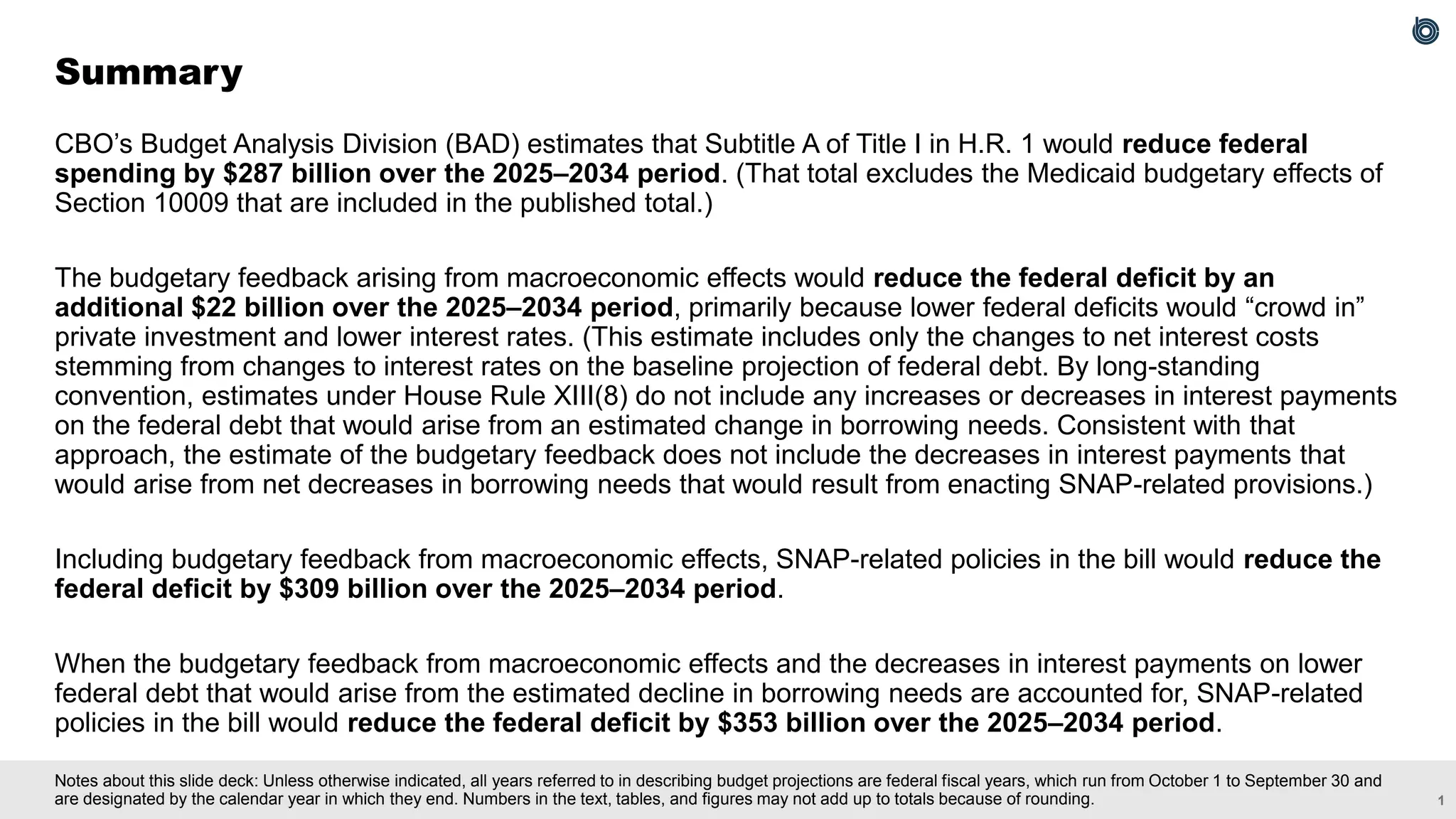
CBO’s Budget Analysis Division (BAD) estimates that Subtitle A of Title I in H.R. 1 would reduce federal
spending by $287 billion over the 2025–2034 period. (That total excludes the Medicaid budgetary effects of
Section 10009 that are included in the published total.)
The budgetary feedback arising from macroeconomic effects would reduce the federal deficit by an
additional $22 billion over the 2025–2034 period, primarily because lower federal deficits would “crowd in”
private investment and lower interest rates. (This estimate includes only the changes to net interest costs
stemming from changes to interest rates on the baseline projection of federal debt. By long-standing
convention, estimates under House Rule XIII(8) do not include any increases or decreases in interest payments
on the federal debt that would arise from an estimated change in borrowing needs. Consistent with that
approach, the estimate of the budgetary feedback does not include the decreases in interest payments that
would arise from net decreases in borrowing needs that would result from enacting SNAP-related provisions.)
Including budgetary feedback from macroeconomic effects, SNAP-related policies in the bill would reduce the
federal deficit by $309 billion over the 2025–2034 period.
When the budgetary feedback from macroeconomic effects and the decreases in interest payments on lower
federal debt that would arise from the estimated decline in borrowing needs are accounted for, SNAP-related
policies in the bill would reduce the federal deficit by $353 billion over the 2025–2034 period.
Summary

2
This slide deck has three sections.
▪ The first section describes the main mechanisms in CBO’s dynamic analysis
(see Slides 3 to 9);
▪ The second section explains the changes to SNAP in H.R. 1
(see Slides 10 to 25); and
▪ The third section explains the macroeconomic effects and budgetary feedback
of changes to SNAP in H.R. 1 (see Slides 26 to 32).
Organization of This Slide Deck

3
Main Mechanisms in
CBO’s Dynamic Analysis

4
Conventional estimates of proposed legislation prepared by CBO and the staff of the
Joint Committee on Taxation (JCT) do account for potential behavioral responses by
households, businesses, and nonfederal governments.
Those conventional estimates do not reflect any changes in the overall size of the
U.S. economy relative to CBO’s baseline macroeconomic projections.
When analyzing proposed major legislation, House Rule XIII(8) requires CBO and JCT to
include the budgetary effects resulting from changes in output, employment, the capital
stock, and other macroeconomic variables, in addition to the behavioral responses in a
conventional estimate.
An analysis of proposed legislation that incorporates such macroeconomic effects is
commonly known as a dynamic analysis.
Conventional Estimates and Dynamic Analysis

5
For more information about the framework CBO uses for evaluating the impact of federal policies on output, see Congressional Budget Office, How CBO Analyzes the Effects of
Changes in Federal Fiscal Policies on the Economy (November 2014), www.cbo.gov/publication/49494.
CBO estimates the macroeconomic effects of changes in federal policies in both the
short term and the longer term:
▪ In the short term, policy changes primarily affect the economy by influencing the
demand for goods and services, which leads to changes in output relative to its potential
(maximum sustainable) level.
– CBO uses its multiplier model to estimate how changes in aggregate demand affect
output. Those demand-side effects are combined with estimates of the policies’
effects on the supply of capital and labor.
▪ In the longer term, changes in policies affect the economy primarily by altering public
saving, federal investment, people’s incentives to work and save, and businesses’
incentive to invest, which leads to changes in potential output.
– CBO uses its Solow-type model in which output is determined by the number of
labor hours that workers supply, the size and composition of the capital stock, and
total factor productivity (TFP).
CBO’s Framework for Estimating Macroeconomic Effects

6
CBO’s multiplier model applies an output multiplier to each policy (or provision), which is
the product of a policy’s direct and indirect effects on aggregate demand. Output
multipliers vary across policies because the direct effects differ.
▪ Direct effects. A policy’s direct effects on aggregate demand result from changes in
purchases by federal agencies and by the people and organizations that receive federal
payments or pay federal taxes. The direct effect on demand is also referred to as the
marginal propensity to consume (MPC).
▪ Indirect effects. Changes in policy affect output indirectly through demand multipliers,
which depend on the response of monetary policy. When output is projected to remain
above its potential and inflation is projected to remain above, or near, the Federal
Reserve’s long-run goal of 2 percent, CBO uses demand multipliers that have a
cumulative effect on output that range from:
– 0.4 to 1.9 over four quarters (central estimate of 1.2), and
– 0.2 to 0.8 over eight quarters (central estimate of 0.5).
CBO’s Multiplier Model and Short-Term Effects on Output

7
For additional details about CBO’s Solow-type model, see Congressional Budget Office, CBO's Policy Growth Model (April 2021), www.cbo.gov/publication/57017.
The nation’s potential to produce goods and services is the key determinant of output over
the long term, so the longer-term effects of changes in policies rely on CBO’s models of
potential output.
CBO’s Solow-type model, or policy growth model, is calibrated to reproduce the agency’s
baseline projection of potential output using an economywide Cobb-Douglas production
function, which depends on the following:
▪ Labor supply defined in terms of economywide potential hours,
▪ Capital services from nonfarm business capital and owner-occupied residential
housing, and
▪ Economywide potential TFP (the average real output per unit of combined labor and
capital services).
CBO’s Solow-Type Model and Longer-Term Effects on Output

8
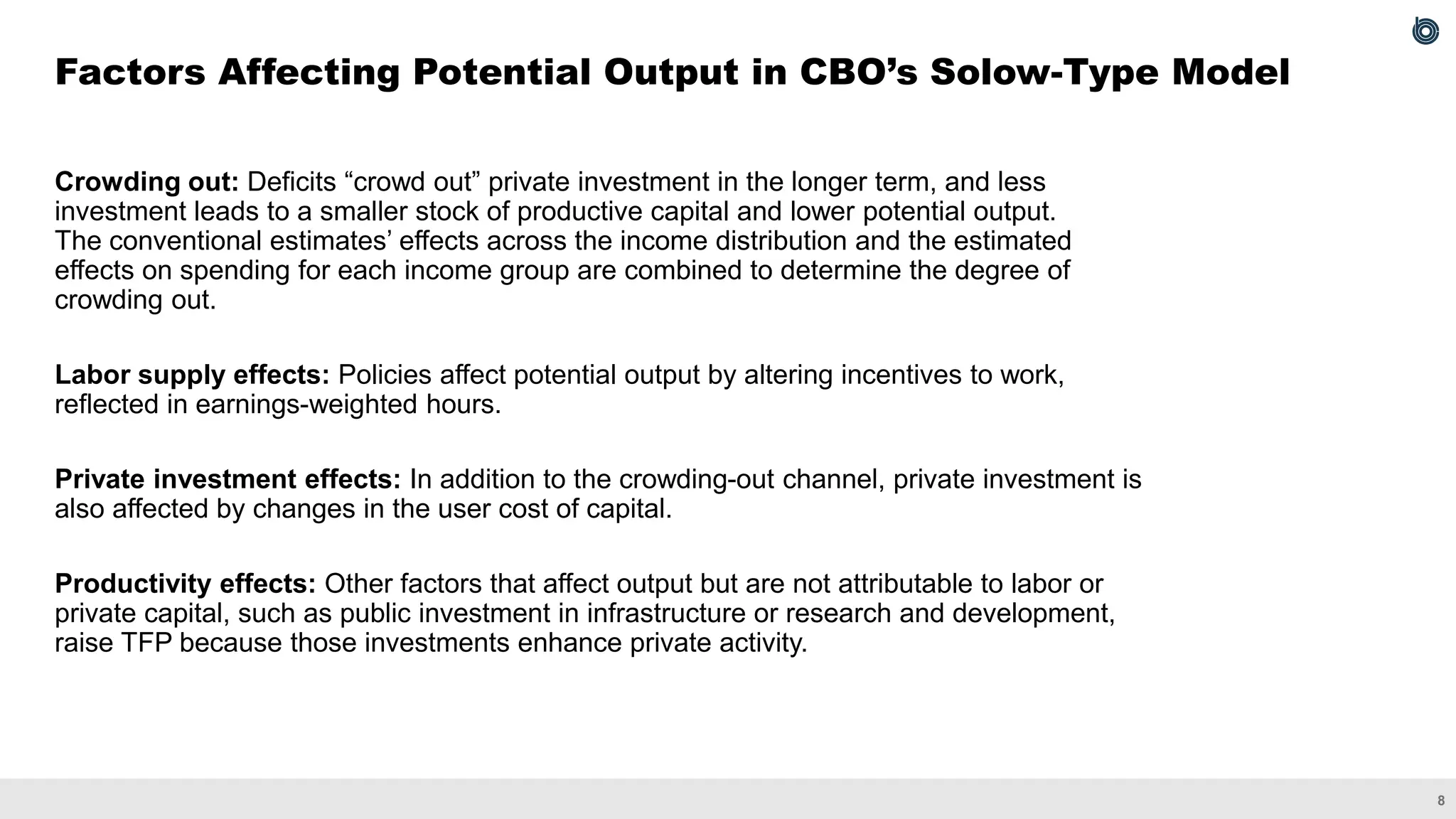
Crowding out: Deficits “crowd out” private investment in the longer term, and less
investment leads to a smaller stock of productive capital and lower potential output.
The conventional estimates’ effects across the income distribution and the estimated
effects on spending for each income group are combined to determine the degree of
crowding out.
Labor supply effects: Policies affect potential output by altering incentives to work,
reflected in earnings-weighted hours.
Private investment effects: In addition to the crowding-out channel, private investment is
also affected by changes in the user cost of capital.
Productivity effects: Other factors that affect output but are not attributable to labor or
private capital, such as public investment in infrastructure or research and development,
raise TFP because those investments enhance private activity.
Factors Affecting Potential Output in CBO’s Solow-Type Model

9
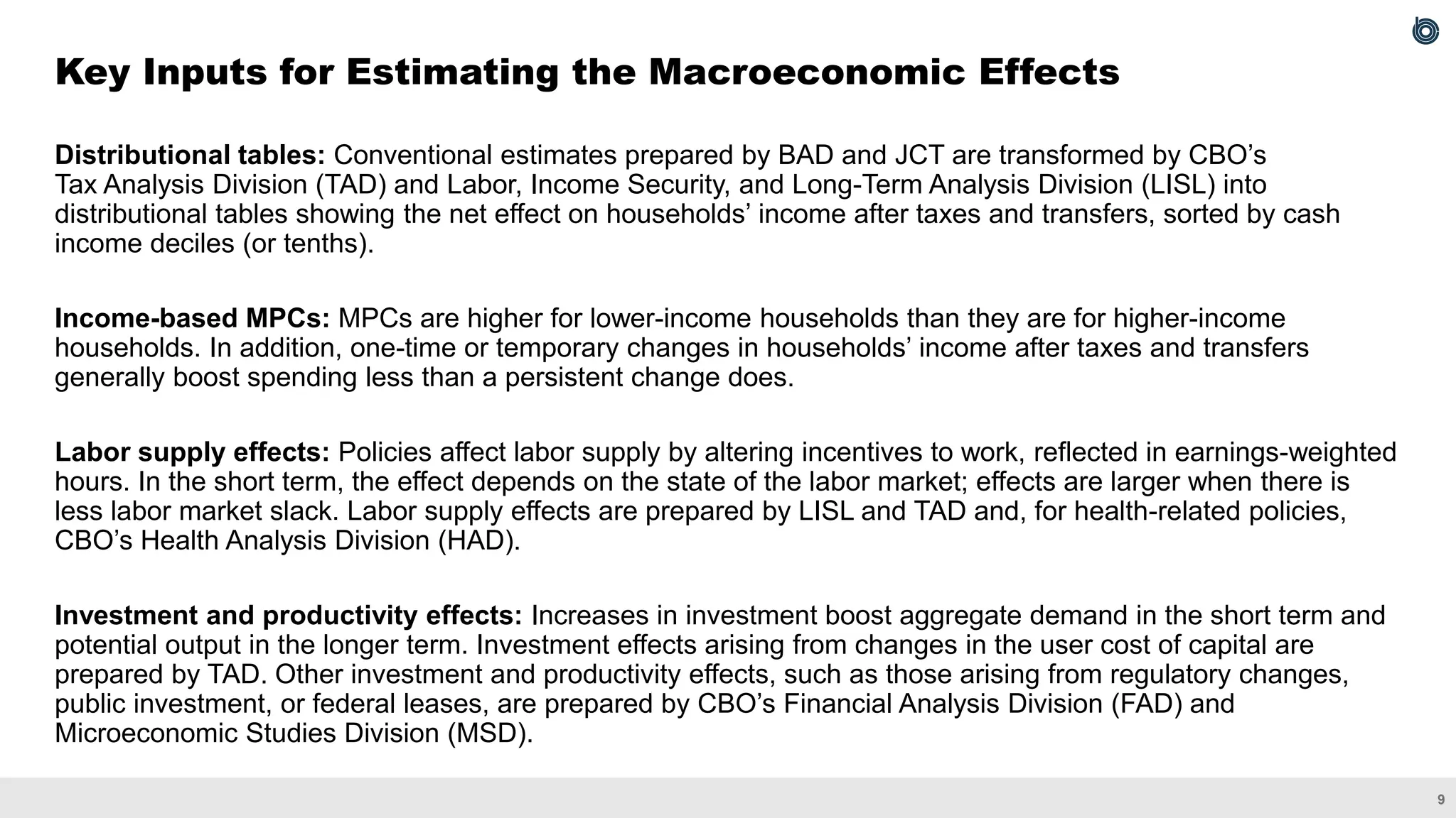
Distributional tables: Conventional estimates prepared by BAD and JCT are transformed by CBO’s
Tax Analysis Division (TAD) and Labor, Income Security, and Long-Term Analysis Division (LISL) into
distributional tables showing the net effect on households’ income after taxes and transfers, sorted by cash
income deciles (or tenths).
Income-based MPCs: MPCs are higher for lower-income households than they are for higher-income
households. In addition, one-time or temporary changes in households’ income after taxes and transfers
generally boost spending less than a persistent change does.
Labor supply effects: Policies affect labor supply by altering incentives to work, reflected in earnings-weighted
hours. In the short term, the effect depends on the state of the labor market; effects are larger when there is
less labor market slack. Labor supply effects are prepared by LISL and TAD and, for health-related policies,
CBO’s Health Analysis Division (HAD).
Investment and productivity effects: Increases in investment boost aggregate demand in the short term and
potential output in the longer term. Investment effects arising from changes in the user cost of capital are
prepared by TAD. Other investment and productivity effects, such as those arising from regulatory changes,
public investment, or federal leases, are prepared by CBO’s Financial Analysis Division (FAD) and
Microeconomic Studies Division (MSD).
Key Inputs for Estimating the Macroeconomic Effects

10
Dynamic Analysis of Changes to
SNAP in H.R. 1

11
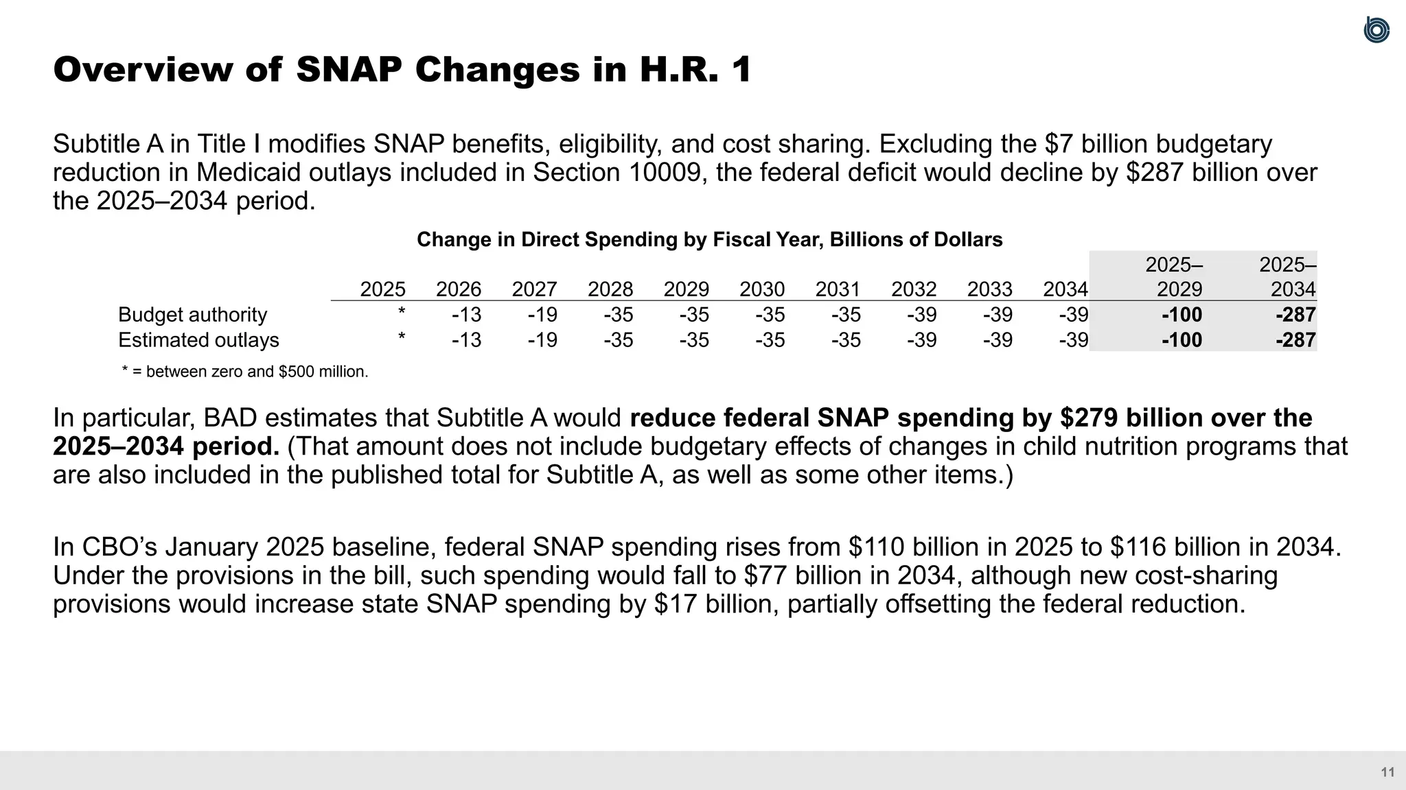
Subtitle A in Title I modifies SNAP benefits, eligibility, and cost sharing. Excluding the $7 billion budgetary
reduction in Medicaid outlays included in Section 10009, the federal deficit would decline by $287 billion over
the 2025–2034 period.
In particular, BAD estimates that Subtitle A would reduce federal SNAP spending by $279 billion over the
2025–2034 period. (That amount does not include budgetary effects of changes in child nutrition programs that
are also included in the published total for Subtitle A, as well as some other items.)
In CBO’s January 2025 baseline, federal SNAP spending rises from $110 billion in 2025 to $116 billion in 2034.
Under the provisions in the bill, such spending would fall to $77 billion in 2034, although new cost-sharing
provisions would increase state SNAP spending by $17 billion, partially offsetting the federal reduction.
Overview of SNAP Changes in H.R. 1
Change in Direct Spending by Fiscal Year, Billions of Dollars
2025 2026 2027 2028 2029 2030 2031 2032 2033 2034
2025–
2029
2025–
2034
Budget authority * -13 -19 -35 -35 -35 -35 -39 -39 -39 -100 -287
Estimated outlays * -13 -19 -35 -35 -35 -35 -39 -39 -39 -100 -287
* = between zero and $500 million.

12
For additional details about each of those provisions, see Congressional Budget Office, letter to the Honorable Amy Klobuchar and the Honorable Angie Craig about the potential
effects on the Supplemental Nutrition Assistance Program of reconciliation recommendations pursuant to H. Con Res. 14 (May 22, 2025), www.cbo.gov/publication/61426.
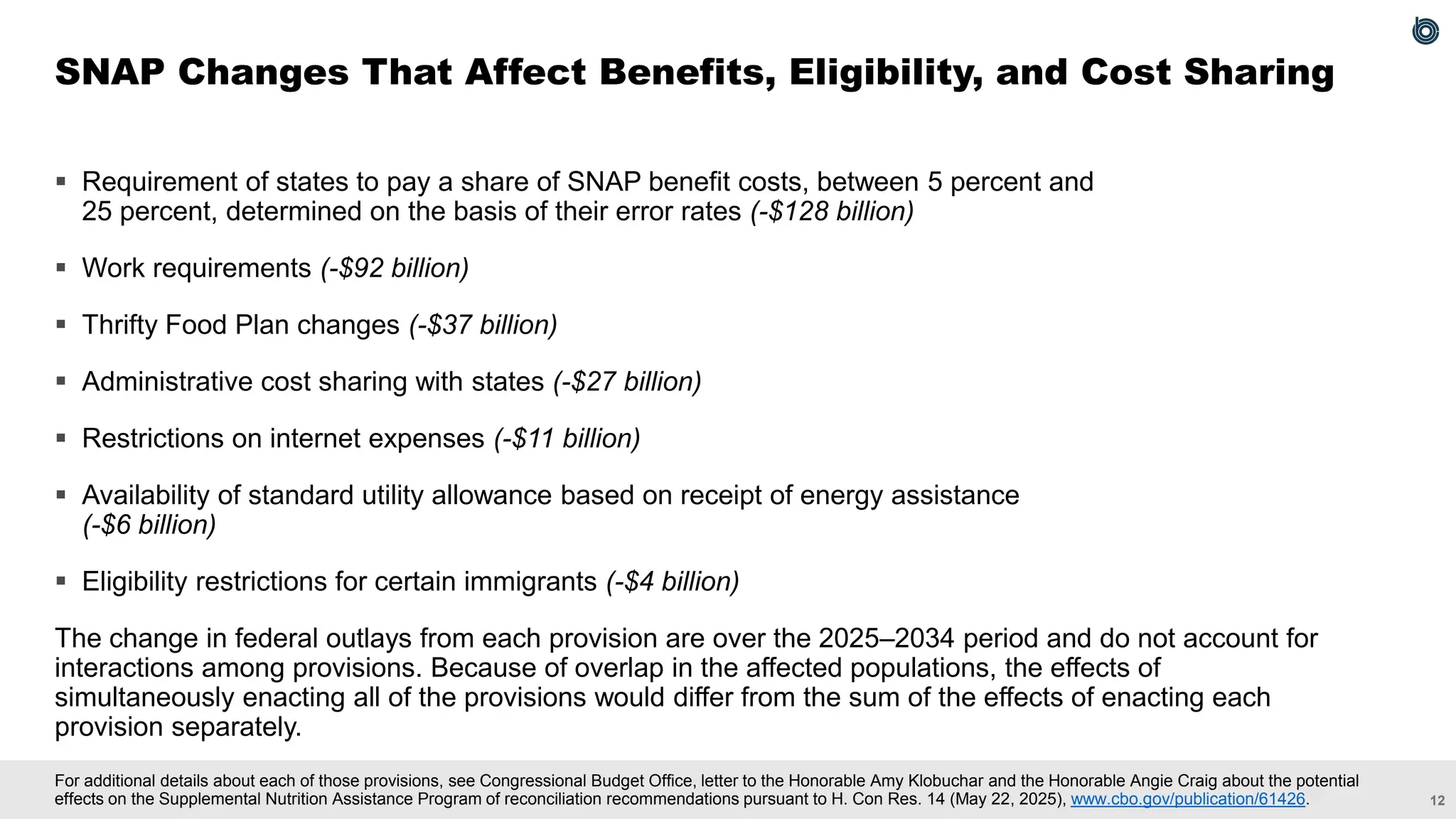
▪ Requirement of states to pay a share of SNAP benefit costs, between 5 percent and
25 percent, determined on the basis of their error rates (-$128 billion)
▪ Work requirements (-$92 billion)
▪ Thrifty Food Plan changes (-$37 billion)
▪ Administrative cost sharing with states (-$27 billion)
▪ Restrictions on internet expenses (-$11 billion)
▪ Availability of standard utility allowance based on receipt of energy assistance
(-$6 billion)
▪ Eligibility restrictions for certain immigrants (-$4 billion)
The change in federal outlays from each provision are over the 2025–2034 period and do not account for
interactions among provisions. Because of overlap in the affected populations, the effects of
simultaneously enacting all of the provisions would differ from the sum of the effects of enacting each
provision separately.
SNAP Changes That Affect Benefits, Eligibility, and Cost Sharing

13
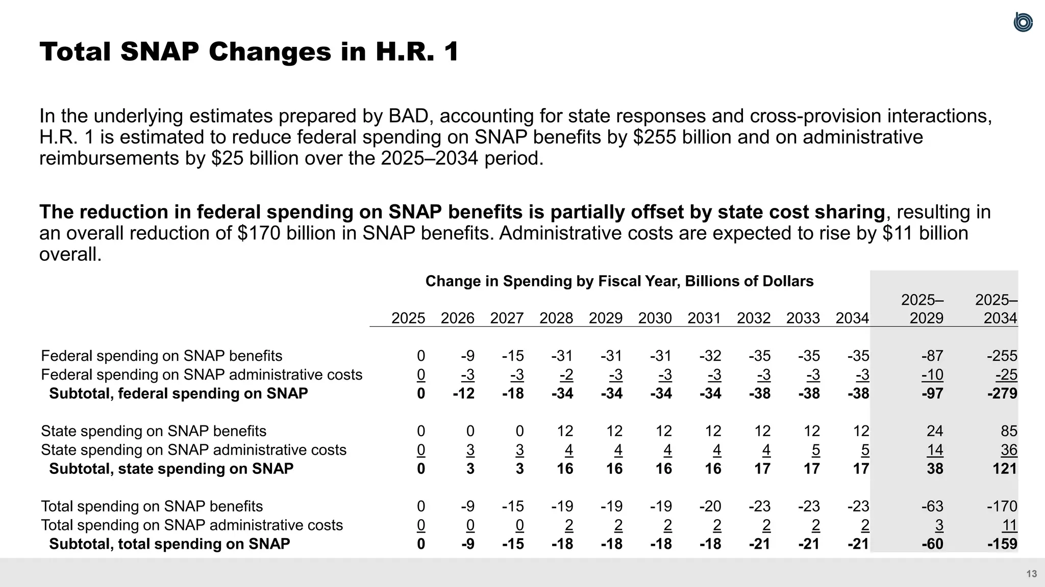
In the underlying estimates prepared by BAD, accounting for state responses and cross-provision interactions,
H.R. 1 is estimated to reduce federal spending on SNAP benefits by $255 billion and on administrative
reimbursements by $25 billion over the 2025–2034 period.
The reduction in federal spending on SNAP benefits is partially offset by state cost sharing, resulting in
an overall reduction of $170 billion in SNAP benefits. Administrative costs are expected to rise by $11 billion
overall.
Total SNAP Changes in H.R. 1
Change in Spending by Fiscal Year, Billions of Dollars
2025 2026 2027 2028 2029 2030 2031 2032 2033 2034
2025–
2029
2025–
2034
Federal spending on SNAP benefits 0 -9 -15 -31 -31 -31 -32 -35 -35 -35 -87 -255
Federal spending on SNAP administrative costs 0 -3 -3 -2 -3 -3 -3 -3 -3 -3 -10 -25
Subtotal, federal spending on SNAP 0 -12 -18 -34 -34 -34 -34 -38 -38 -38 -97 -279
State spending on SNAP benefits 0 0 0 12 12 12 12 12 12 12 24 85
State spending on SNAP administrative costs 0 3 3 4 4 4 4 4 5 5 14 36
Subtotal, state spending on SNAP 0 3 3 16 16 16 16 17 17 17 38 121
Total spending on SNAP benefits 0 -9 -15 -19 -19 -19 -20 -23 -23 -23 -63 -170
Total spending on SNAP administrative costs 0 0 0 2 2 2 2 2 2 2 3 11
Subtotal, total spending on SNAP 0 -9 -15 -18 -18 -18 -18 -21 -21 -21 -60 -159

14
BAD’s conventional estimates already reflect state responses within programs, but the net
change in states’ fiscal positions, beyond the directly affected programs, is generally not
accounted for.
For example, CBO expects that some states would maintain current SNAP benefits and eligibility
and that others would modify benefits or eligibility or possibly leave the program altogether. The
agency estimated state responses in the aggregate using a probabilistic approach to account for
a range of possible outcomes.
If a change in federal policy resulted in a change to a state’s fiscal position relative to what would
occur under current law, how states reacted to that change would depend on whether the federal
policy generated a surplus or a deficit. It could also depend on the time horizon, with states
shifting from an initial short-term response (such as relying on rainy day funds until they can fully
adjust) to a longer-term source of financing.
States would certainly vary how they respond to a change in their fiscal position. CBO typically
estimates state responses in the aggregate, accounting for a range of possible outcomes.
How State Responses Were Prepared

15
For the agency’s short-term estimates of the initial impact on state budgets, CBO used
the findings in Rueben, Randall, and Boddupalli (2018), which followed a similar empirical
approach to that of Poterba (1994) and Clemens and Miran (2012), to determine how
states adjusted their revenues, expenditures, and (implicitly) their other means of financing
in response to an immediate change in their fiscal position.
In that analysis, they found that from 1990 to 2015:
▪ When states experienced a $1 deficit shock, they typically reduced spending by
$0.26 and increased revenues by $0.08 in the current year. They increased revenues by
an additional $0.14 in the following year.
▪ When states experienced a $1 surplus shock, they generally made no change to
spending, reduced revenues by $0.04 in the current year, and further reduced revenues
by $0.08 in the following year.
State Government Responses in the Short Term

16
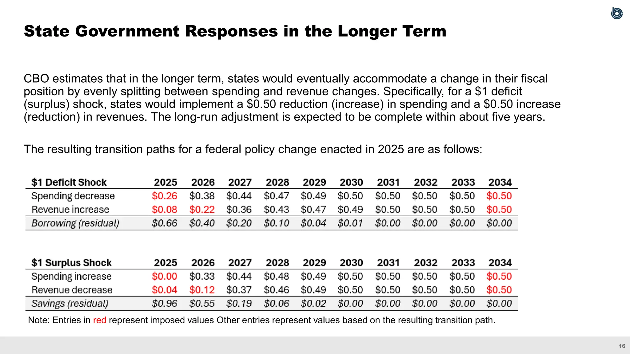
CBO estimates that in the longer term, states would eventually accommodate a change in their fiscal
position by evenly splitting between spending and revenue changes. Specifically, for a $1 deficit
(surplus) shock, states would implement a $0.50 reduction (increase) in spending and a $0.50 increase
(reduction) in revenues. The long-run adjustment is expected to be complete within about five years.
The resulting transition paths for a federal policy change enacted in 2025 are as follows:
State Government Responses in the Longer Term
Note: Entries in red represent imposed values Other entries represent values based on the resulting transition path.

17
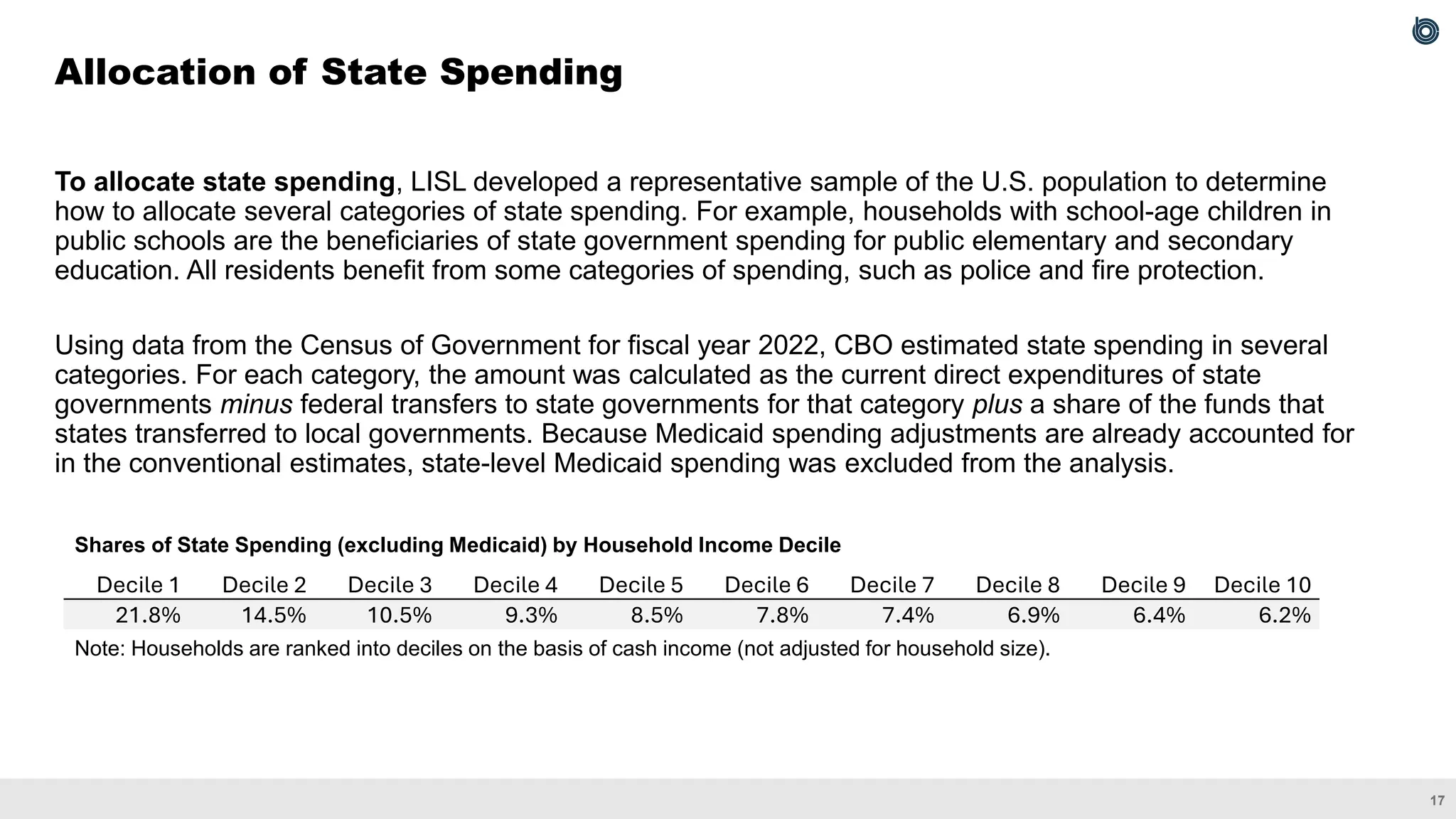
To allocate state spending, LISL developed a representative sample of the U.S. population to determine
how to allocate several categories of state spending. For example, households with school-age children in
public schools are the beneficiaries of state government spending for public elementary and secondary
education. All residents benefit from some categories of spending, such as police and fire protection.
Using data from the Census of Government for fiscal year 2022, CBO estimated state spending in several
categories. For each category, the amount was calculated as the current direct expenditures of state
governments minus federal transfers to state governments for that category plus a share of the funds that
states transferred to local governments. Because Medicaid spending adjustments are already accounted for
in the conventional estimates, state-level Medicaid spending was excluded from the analysis.
Allocation of State Spending
Decile 1 Decile 2 Decile 3 Decile 4 Decile 5 Decile 6 Decile 7 Decile 8 Decile 9 Decile 10
21.8% 14.5% 10.5% 9.3% 8.5% 7.8% 7.4% 6.9% 6.4% 6.2%
Shares of State Spending (excluding Medicaid) by Household Income Decile
Note: Households are ranked into deciles on the basis of cash income (not adjusted for household size).

18
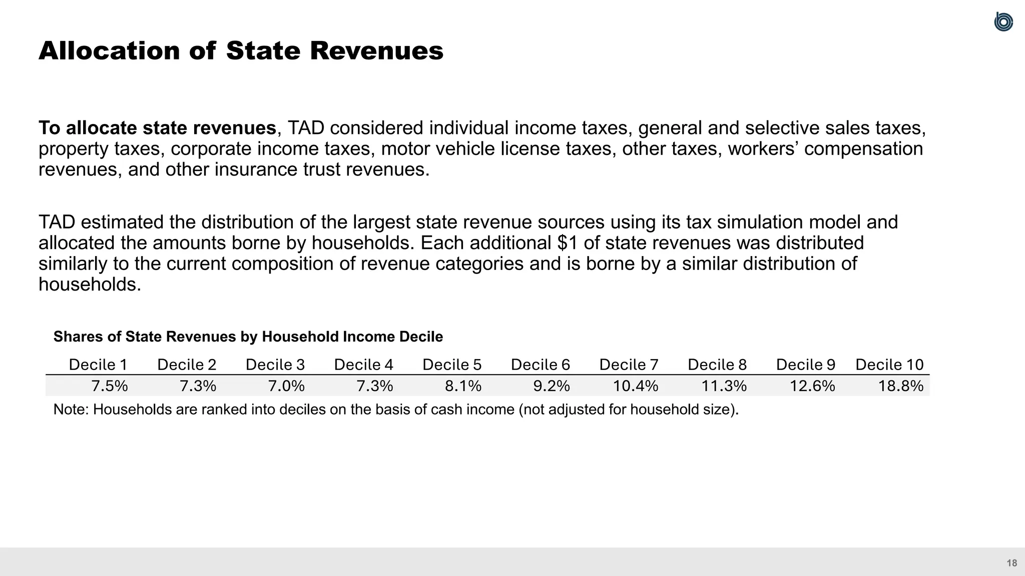
To allocate state revenues, TAD considered individual income taxes, general and selective sales taxes,
property taxes, corporate income taxes, motor vehicle license taxes, other taxes, workers’ compensation
revenues, and other insurance trust revenues.
TAD estimated the distribution of the largest state revenue sources using its tax simulation model and
allocated the amounts borne by households. Each additional $1 of state revenues was distributed
similarly to the current composition of revenue categories and is borne by a similar distribution of
households.
Allocation of State Revenues
Decile 1 Decile 2 Decile 3 Decile 4 Decile 5 Decile 6 Decile 7 Decile 8 Decile 9 Decile 10
7.5% 7.3% 7.0% 7.3% 8.1% 9.2% 10.4% 11.3% 12.6% 18.8%
Shares of State Revenues by Household Income Decile
Note: Households are ranked into deciles on the basis of cash income (not adjusted for household size).

19
For more details about how the agency projects that states would respond to changes in Medicaid policies, see Congressional Budget Office, letter to the Honorable Ron Wyden and
the Honorable Frank Pallone, Jr. providing estimates for Medicaid policy options and state responses (May 7, 2025), www.cbo.gov/publication/61377.
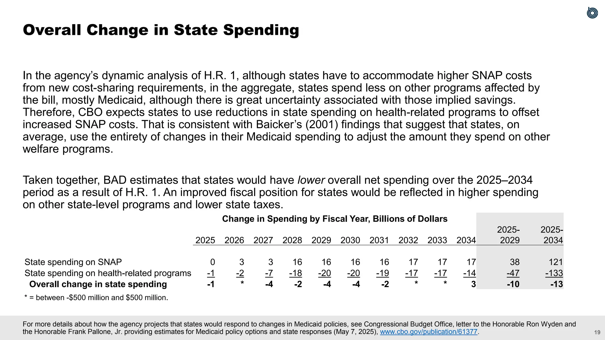
In the agency’s dynamic analysis of H.R. 1, although states have to accommodate higher SNAP costs
from new cost-sharing requirements, in the aggregate, states spend less on other programs affected by
the bill, mostly Medicaid, although there is great uncertainty associated with those implied savings.
Therefore, CBO expects states to use reductions in state spending on health-related programs to offset
increased SNAP costs. That is consistent with Baicker’s (2001) findings that suggest that states, on
average, use the entirety of changes in their Medicaid spending to adjust the amount they spend on other
welfare programs.
Taken together, BAD estimates that states would have lower overall net spending over the 2025–2034
period as a result of H.R. 1. An improved fiscal position for states would be reflected in higher spending
on other state-level programs and lower state taxes.
Overall Change in State Spending
Change in Spending by Fiscal Year, Billions of Dollars
2025 2026 2027 2028 2029 2030 2031 2032 2033 2034
2025-
2029
2025-
2034
State spending on SNAP 0 3 3 16 16 16 16 17 17 17 38 121
State spending on health-related programs -1 -2 -7 -18 -20 -20 -19 -17 -17 -14 -47 -133
Overall change in state spending -1 * -4 -2 -4 -4 -2 * * 3 -10 -13
* = between -$500 million and $500 million.

20
Aggregate demand effects
▪ The distributional table includes the total (federal + state) change in SNAP benefits as well states’
fiscal responses. Changes in administrative costs are treated as government consumption.
Labor supply effects
▪ SNAP recipients would adjust their labor supply in response to the change in benefit amounts and
changes in eligibility, such as work requirements.
▪ Workers would adjust their labor supply in response to changes in state labor income taxes.
Although the labor supply effects could have been attributed to the Medicaid provisions in H.R. 1,
they were attributed to the SNAP provisions for illustrative purposes to demonstrate how states’
responses influence labor supply in CBO’s dynamic analysis.
Investment effects
▪ SNAP provisions in H.R. 1 would reduce the federal deficit and would crowd in private investment.
States might also respond by changing capital income taxes, which would impact the user cost of
capital and, in turn, private investment.
Estimating the Macroeconomic Effects of SNAP Changes in H.R. 1

21
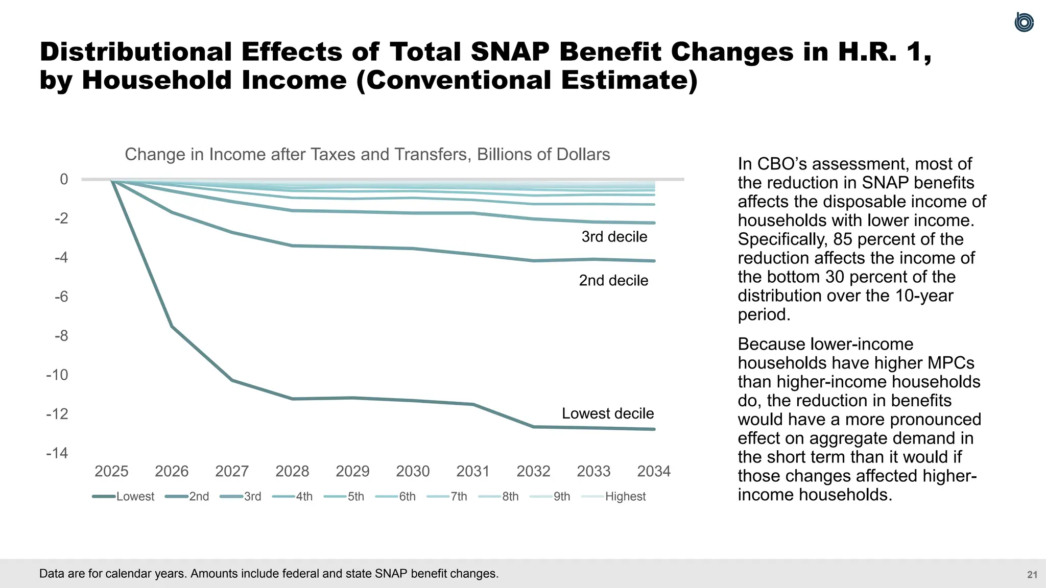
Data are for calendar years. Amounts include federal and state SNAP benefit changes.
Distributional Effects of Total SNAP Benefit Changes in H.R. 1,
by Household Income (Conventional Estimate)
-14
-12
-10
-8
-6
-4
-2
0
2025 2026 2027 2028 2029 2030 2031 2032 2033 2034
Change in Income after Taxes and Transfers, Billions of Dollars
Lowest 2nd 3rd 4th 5th 6th 7th 8th 9th Highest
Lowest decile
2nd decile
3rd decile
In CBO’s assessment, most of
the reduction in SNAP benefits
affects the disposable income of
households with lower income.
Specifically, 85 percent of the
reduction affects the income of
the bottom 30 percent of the
distribution over the 10-year
period.
Because lower-income
households have higher MPCs
than higher-income households
do, the reduction in benefits
would have a more pronounced
effect on aggregate demand in
the short term than it would if
those changes affected higher-
income households.

22
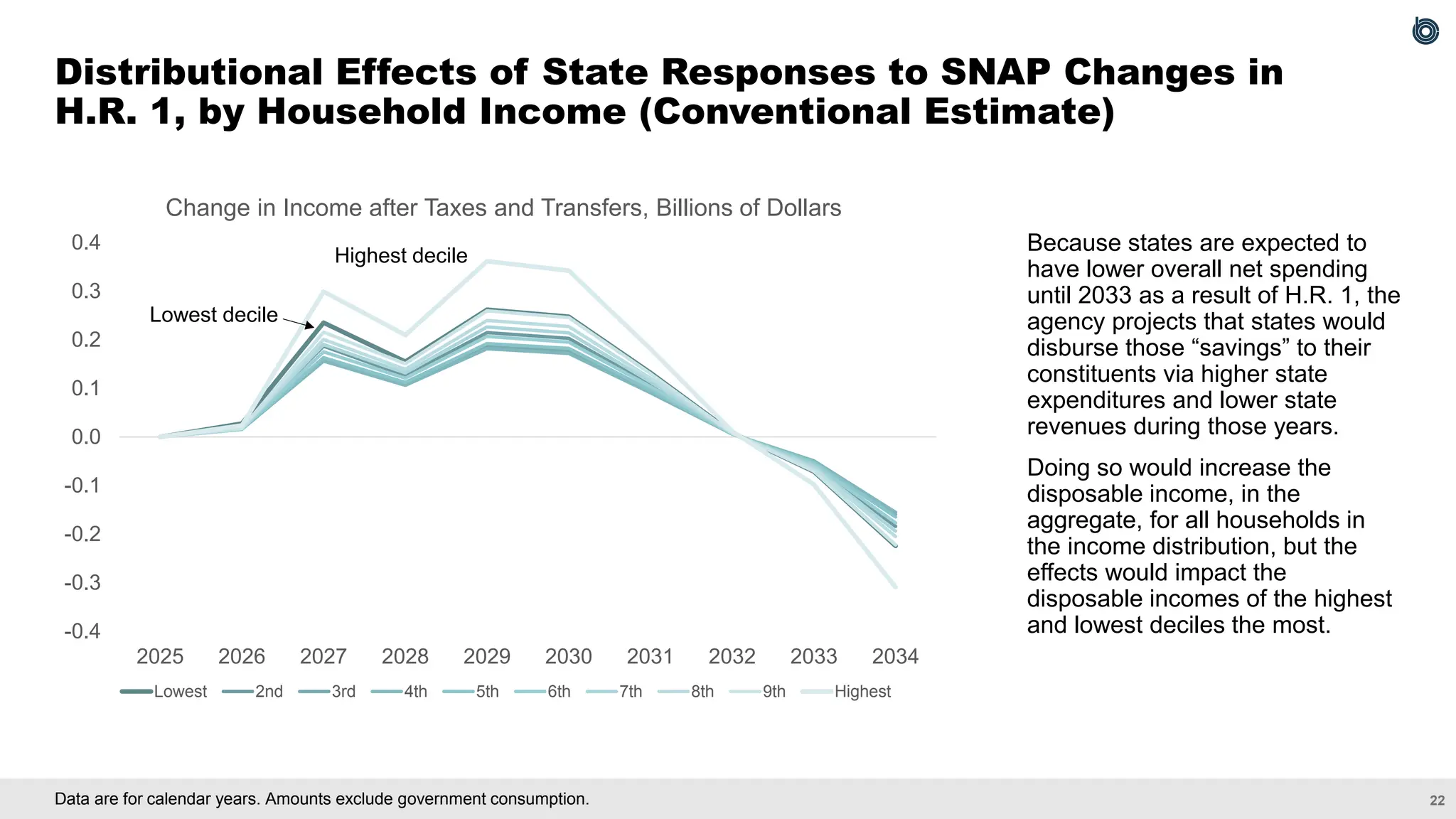
Data are for calendar years. Amounts exclude government consumption.
Distributional Effects of State Responses to SNAP Changes in
H.R. 1, by Household Income (Conventional Estimate)
Because states are expected to
have lower overall net spending
until 2033 as a result of H.R. 1, the
agency projects that states would
disburse those “savings” to their
constituents via higher state
expenditures and lower state
revenues during those years.
Doing so would increase the
disposable income, in the
aggregate, for all households in
the income distribution, but the
effects would impact the
disposable incomes of the highest
and lowest deciles the most.
-0.4
-0.3
-0.2
-0.1
0.0
0.1
0.2
0.3
0.4
2025 2026 2027 2028 2029 2030 2031 2032 2033 2034
Change in Income after Taxes and Transfers, Billions of Dollars
Lowest 2nd 3rd 4th 5th 6th 7th 8th 9th Highest
Highest decile
Lowest decile

23
Labor Supply Effects of SNAP Changes in H.R. 1
1. LISL estimates that SNAP recipients would increase their labor supply in response to
the reduction in benefits and changes in eligibility, resulting in an increase of 0.02%
of earnings-weighted hours by 2034.
2. If the SNAP changes were enacted on their own, other workers would be expected to
decrease their labor supply in response to the higher state labor income taxes that
would be needed to finance the additional state SNAP expenditures. However, on net,
the bill as a whole is estimated to result in lower state spending in most years over the
2025–2034 period, mainly because of the changes to Medicaid as well as states’
expected response to those changes. Taken together, TAD estimates that the
decrease in state labor income taxes would generate a slight increase in
earnings-weighted hours until 2033.

24
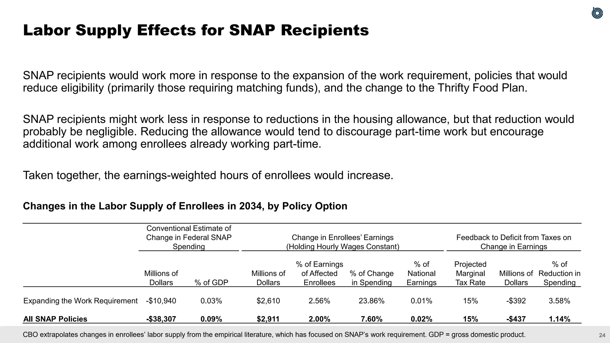
CBO extrapolates changes in enrollees’ labor supply from the empirical literature, which has focused on SNAP’s work requirement. GDP = gross domestic product.
SNAP recipients would work more in response to the expansion of the work requirement, policies that would
reduce eligibility (primarily those requiring matching funds), and the change to the Thrifty Food Plan.
SNAP recipients might work less in response to reductions in the housing allowance, but that reduction would
probably be negligible. Reducing the allowance would tend to discourage part-time work but encourage
additional work among enrollees already working part-time.
Taken together, the earnings-weighted hours of enrollees would increase.
Changes in the Labor Supply of Enrollees in 2034, by Policy Option
Labor Supply Effects for SNAP Recipients
Conventional Estimate of
Change in Federal SNAP
Spending
Change in Enrollees’ Earnings
(Holding Hourly Wages Constant)
Feedback to Deficit from Taxes on
Change in Earnings
Millions of
Dollars % of GDP
Millions of
Dollars
% of Earnings
of Affected
Enrollees
% of Change
in Spending
% of
National
Earnings
Projected
Marginal
Tax Rate
Millions of
Dollars
% of
Reduction in
Spending
Expanding the Work Requirement -$10,940 0.03% $2,610 2.56% 23.86% 0.01% 15% -$392 3.58%
All SNAP Policies -$38,307 0.09% $2,911 2.00% 7.60% 0.02% 15% -$437 1.14%

25
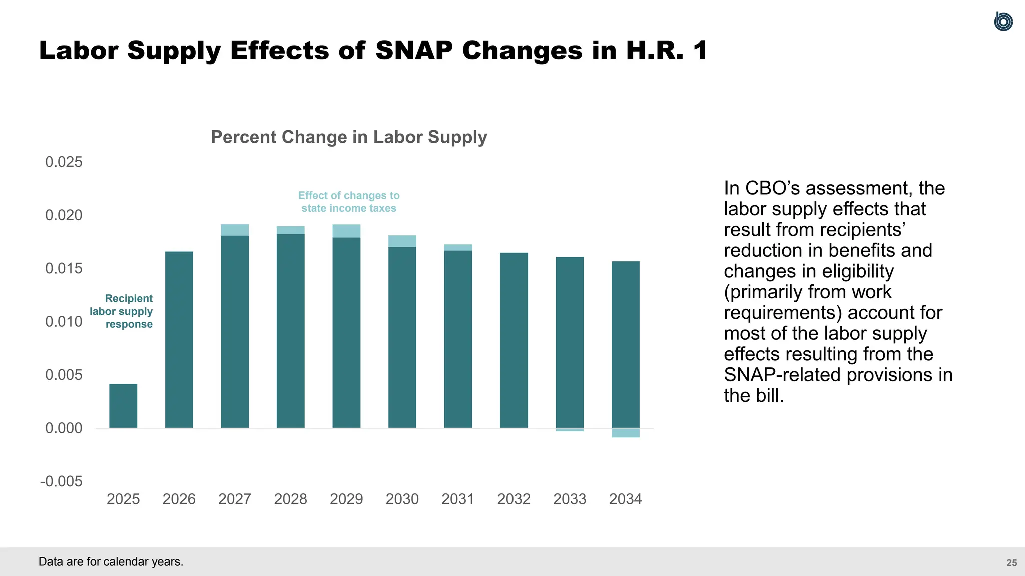
Data are for calendar years.
Labor Supply Effects of SNAP Changes in H.R. 1
In CBO’s assessment, the
labor supply effects that
result from recipients’
reduction in benefits and
changes in eligibility
(primarily from work
requirements) account for
most of the labor supply
effects resulting from the
SNAP-related provisions in
the bill.
-0.005
0.000
0.005
0.010
0.015
0.020
0.025
2025 2026 2027 2028 2029 2030 2031 2032 2033 2034
Percent Change in Labor Supply
Effect of changes to
state income taxes
Recipient
labor supply
response

26
Macroeconomic Effects and
Budgetary Feedback of Changes to
SNAP in H.R. 1

27
Data are for calendar years. For more information about CBO’s transition between short-term and longer-term effects, see Congressional Budget Office, How CBO Analyzes the
Effects of Changes in Federal Fiscal Policies on the Economy (November 2014), www.cbo.gov/publication/49494.
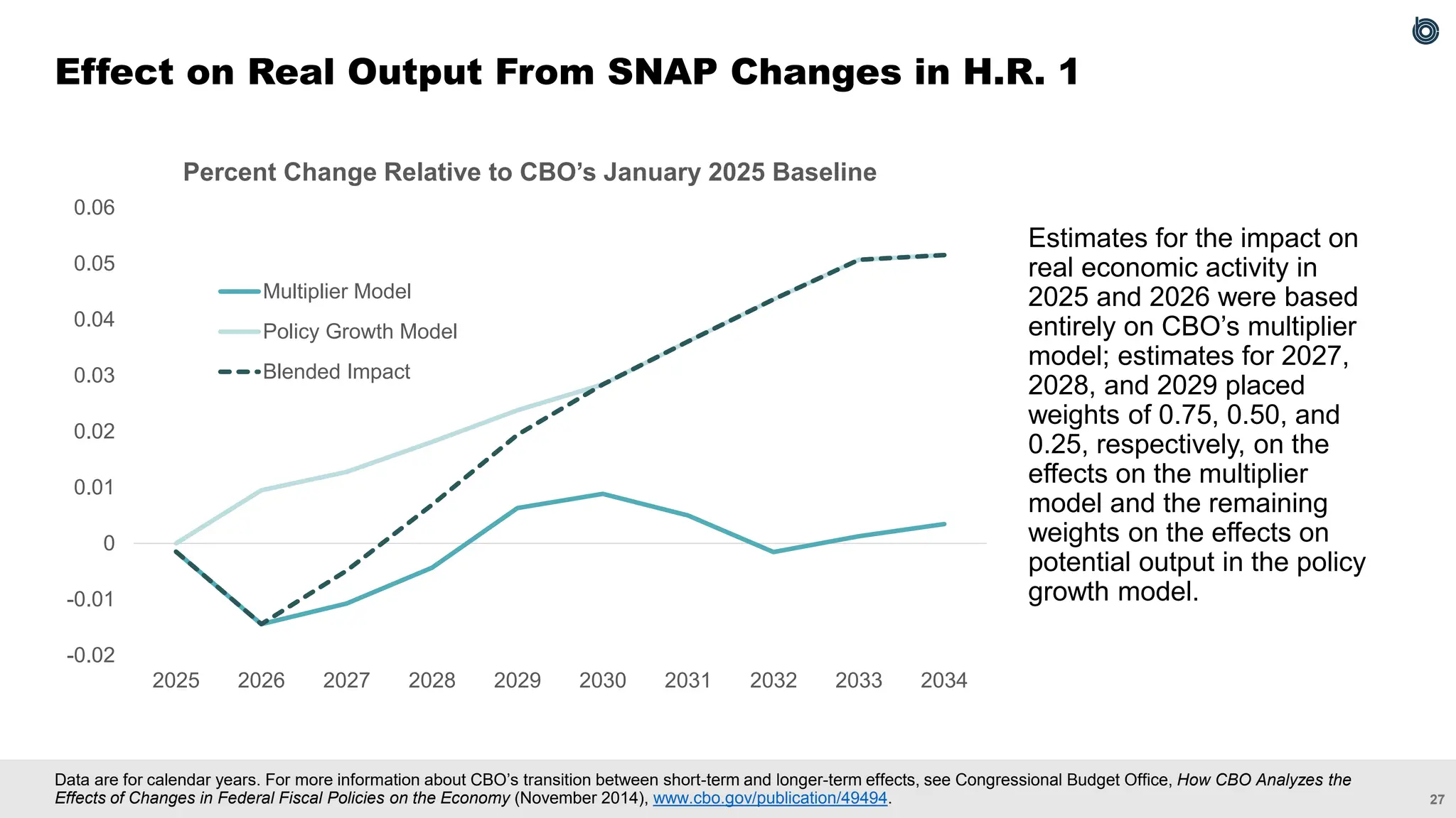
Effect on Real Output From SNAP Changes in H.R. 1
Estimates for the impact on
real economic activity in
2025 and 2026 were based
entirely on CBO’s multiplier
model; estimates for 2027,
2028, and 2029 placed
weights of 0.75, 0.50, and
0.25, respectively, on the
effects on the multiplier
model and the remaining
weights on the effects on
potential output in the policy
growth model.
-0.02
-0.01
0
0.01
0.02
0.03
0.04
0.05
0.06
2025 2026 2027 2028 2029 2030 2031 2032 2033 2034
Percent Change Relative to CBO’s January 2025 Baseline
Multiplier Model
Policy Growth Model
Blended Impact

28
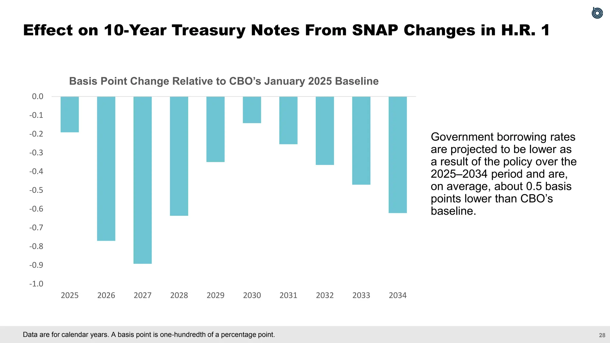
Data are for calendar years. A basis point is one-hundredth of a percentage point.
Effect on 10-Year Treasury Notes From SNAP Changes in H.R. 1
Government borrowing rates
are projected to be lower as
a result of the policy over the
2025–2034 period and are,
on average, about 0.5 basis
points lower than CBO’s
baseline.
-1.0
-0.9
-0.8
-0.7
-0.6
-0.5
-0.4
-0.3
-0.2
-0.1
0.0
2025 2026 2027 2028 2029 2030 2031 2032 2033 2034
Basis Point Change Relative to CBO’s January 2025 Baseline

29
For more details on CBO’s dynamic analysis of all the provisions in H.R. 1, see Congressional Budget Office, H.R. 1, One Big Beautiful Bill Act (Dynamic Estimate) (June 17, 2025),
www.cbo.gov/publication/61486.
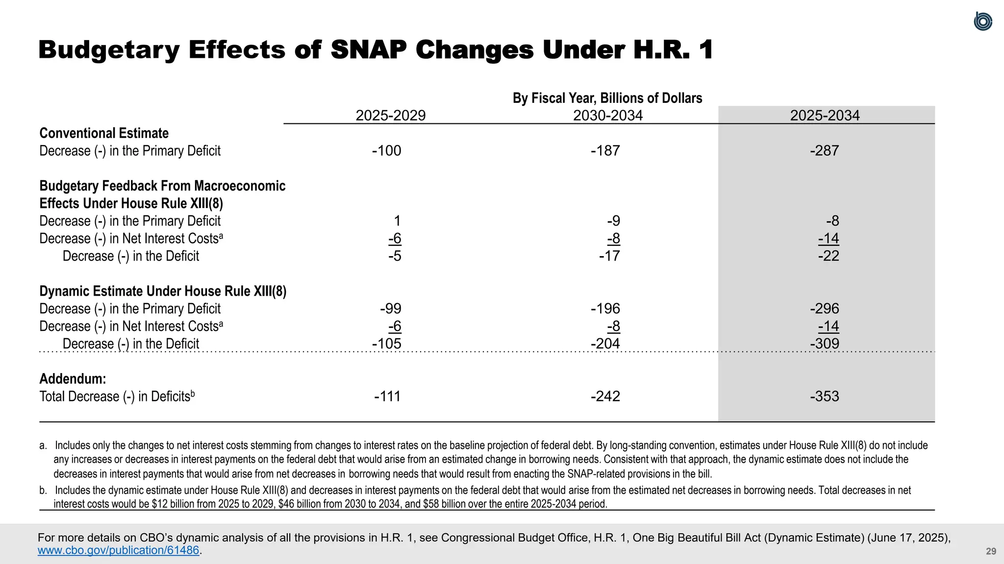
Budgetary Effects of SNAP Changes Under H.R. 1
By Fiscal Year, Billions of Dollars
2025-2029 2030-2034 2025-2034
Conventional Estimate
Decrease (-) in the Primary Deficit -100 -187 -287
Budgetary Feedback From Macroeconomic
Effects Under House Rule XIII(8)
Decrease (-) in the Primary Deficit 1 -9 -8
Decrease (-) in Net Interest Costsa -6 -8 -14
Decrease (-) in the Deficit -5 -17 -22
Dynamic Estimate Under House Rule XIII(8)
Decrease (-) in the Primary Deficit -99 -196 -296
Decrease (-) in Net Interest Costsa -6 -8 -14
Decrease (-) in the Deficit -105 -204 -309
Addendum:
Total Decrease (-) in Deficitsb -111 -242 -353
a. Includes only the changes to net interest costs stemming from changes to interest rates on the baseline projection of federal debt. By long-standing convention, estimates under House Rule XIII(8) do not include
any increases or decreases in interest payments on the federal debt that would arise from an estimated change in borrowing needs. Consistent with that approach, the dynamic estimate does not include the
decreases in interest payments that would arise from net decreases in borrowing needs that would result from enacting the SNAP-related provisions in the bill.
b. Includes the dynamic estimate under House Rule XIII(8) and decreases in interest payments on the federal debt that would arise from the estimated net decreases in borrowing needs. Total decreases in net
interest costs would be $12 billion from 2025 to 2029, $46 billion from 2030 to 2034, and $58 billion over the entire 2025-2034 period.

30
Effects on Net Interest
Excluding the effects of Section 10009, which affects Medicaid outlays, CBO estimates that SNAP-
related provisions in H.R. 1 would reduce the primary deficit by $287 billion over the 2025–2034 period.
The budgetary feedback stemming from the SNAP-related policies in the bill’s effects on the economy
would further reduce the primary deficit by $8 billion over that period, partially because lower deficits
would cause private investment and output to be higher. However, the largest source of feedback savings
is lower interest costs because of lower interest rates, driven by the crowding in of private capital.
In CBO’s assessment, the reduction in federal budget deficits over the 2025–2034 period increases
private investment by crowding in private capital. In addition to the longer-term effects of reduced federal
borrowing on interest rates, higher private investment raises the amount of capital per worker, which
lowers the return on capital and contributes to the decline in interest rates. When lower net interest costs
stemming from changes to interest rates on the baseline projection of federal debt are taken into
account, the deficit would be reduced by an additional $14 billion.
When the dynamic estimate under House Rule XIII(8) and the decreases in interest payments on the
federal debt that would arise from the estimated net decreases in borrowing needs are accounted for,
total net interest costs would be $58 billion lower over the period.

31
In CBO’s macroeconomic forecast, the average interest rate on federal debt generally
increases by 2 basis points in the long term for each percentage-point increase in debt held by
the public as a share of gross domestic product (GDP). For the basis of that estimate, and
CBO’s recent reduction of it from 2.5 basis points to 2 basis points, see Neveu and Schafer
(2024).
To align the results with CBO’s forecasting model, CBO has increased the long-term sensitivity
of interest rates to federal debt in its fiscal policy analysis, including in its dynamic analysis of
H.R. 1.
CBO’s fiscal policy analysis has previously used a model in which the interest rate on 10-year
Treasury notes had a one-to-one relationship with the return on capital in the long term (CBO
2021). That relationship resulted in lower sensitivity of interest rates to changes in federal debt,
which differed from the responses implied by the framework CBO used to incorporate
legislative changes into its macroeconomic forecast. That lower sensitivity is the primary
reason that interest rate responses in previous analyses have been smaller. (For an example
of one earlier analysis with a smaller response, see CBO 2024.)
Sensitivity of Interest Rates to Changes in Federal Debt

32
SNAP-related provisions in the bill are expected to lower output in the short term because of benefit
reductions for households with lower income but boost output because the labor supply and private
investment would be larger, on net, in the longer term.
After incorporating macroeconomic feedback and savings from reduced net interest costs from
lower federal debt, SNAP-related policies in H.R. 1 would reduce the federal deficit by a total of
$353 billion over the 2025–2034 period.
Current areas of uncertainty
▪ Because many policies begin to take effect in 2027 and beyond, CBO’s projected transition
between the short term and longer term mitigates the demand-side effects beginning in that year.
However, the change in demand of households and businesses may vary considerably over time.
▪ The self-financing of states is subject to considerable uncertainty. States, on average, may
respond to a lesser or greater extent than CBO currently anticipates. In addition, aggregating state
behavior may mask important differences at the state level.
Dynamic Effects of SNAP Provisions in H.R. 1

33
Katherine Baicker, “Government Decision-Making and the Incidence of Federal Mandates,”
Journal of Public Economics, vol. 82, no. 2 (November 2001), pp. 147–194,
https://doi.org/10.1016/S0047-2727(00)00149-3.
Jeffrey Clemens and Stephen Miran, “Fiscal Policy Multipliers on Subnational Government
Spending,” American Economic Journal: Economic Policy, vol. 4, no. 2 (May 2012), pp. 46–68,
https://doi.org/10.1257/pol.4.2.46.
Congressional Budget Office, “CBO’s Policy Growth Model” (April 2021), Slide 9,
Congressional Budget Office, “How the Expiring Individual Income Tax Provisions in the 2017
Tax Act Affect CBO’s Economic Forecast” (December 2024) Slide 15,
References

34
Andre R. Neveu and Jeffrey Schafer, Revisiting the Relationship Between Debt
and Long-Term Interest Rates: Working Paper 2024-05 (Congressional Budget
Office, December 2024), www.cbo.gov/publication/60314.
James M. Poterba, “State Responses to Fiscal Crises: The Effects of Budgetary
Institutions and Politics,” Journal of Political Economy, vol. 102, no. 4 (August
1994), pp. 799–821, https://doi.org/10.1086/261955.
Kim S. Rueben, Megan Randall, and Aravind Boddupalli, Budget Processes and
the Great Recession: How State Fiscal Institutions Shape Tax and Spending
Decisions. (Urban Institute, October 2018), https://tinyurl.com/yurrkfza.
References (Continued)

35
This document was prepared to enhance the transparency of the work of the
Congressional Budget Office and to encourage external review of that work. In
keeping with CBO’s mandate to provide objective, impartial analysis, it makes no
recommendations.
The document is the result of work by analysts across CBO. It was reviewed by
Devrim Demirel, Mark Hadley, Jeffrey Kling, John McClelland, Sam Papenfuss,
and Julie Topoleski.
CBO seeks feedback to make its work as useful as possible. Please send
comments to communications@cbo.gov.
About This Document

Dynamic Analysis of Changes to the Supplemental Nutrition Assistance Program (SNAP) in H.R. 1

More Related Content

Similar to Dynamic Analysis of Changes to the Supplemental Nutrition Assistance Program (SNAP) in H.R. 1

More from Congressional Budget Office

Recently uploaded

Dynamic Analysis of Changes to the Supplemental Nutrition Assistance Program (SNAP) in H.R. 1