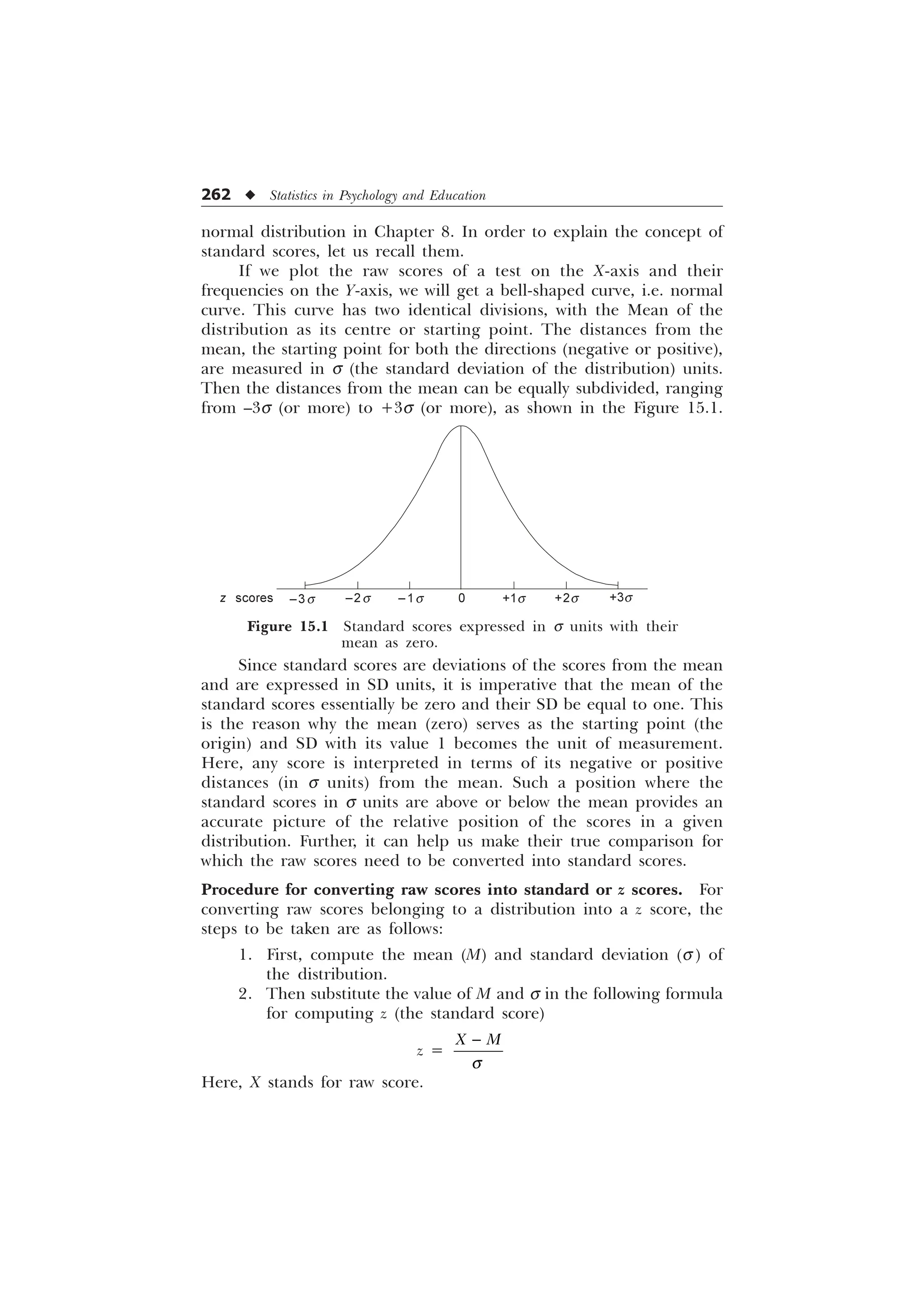
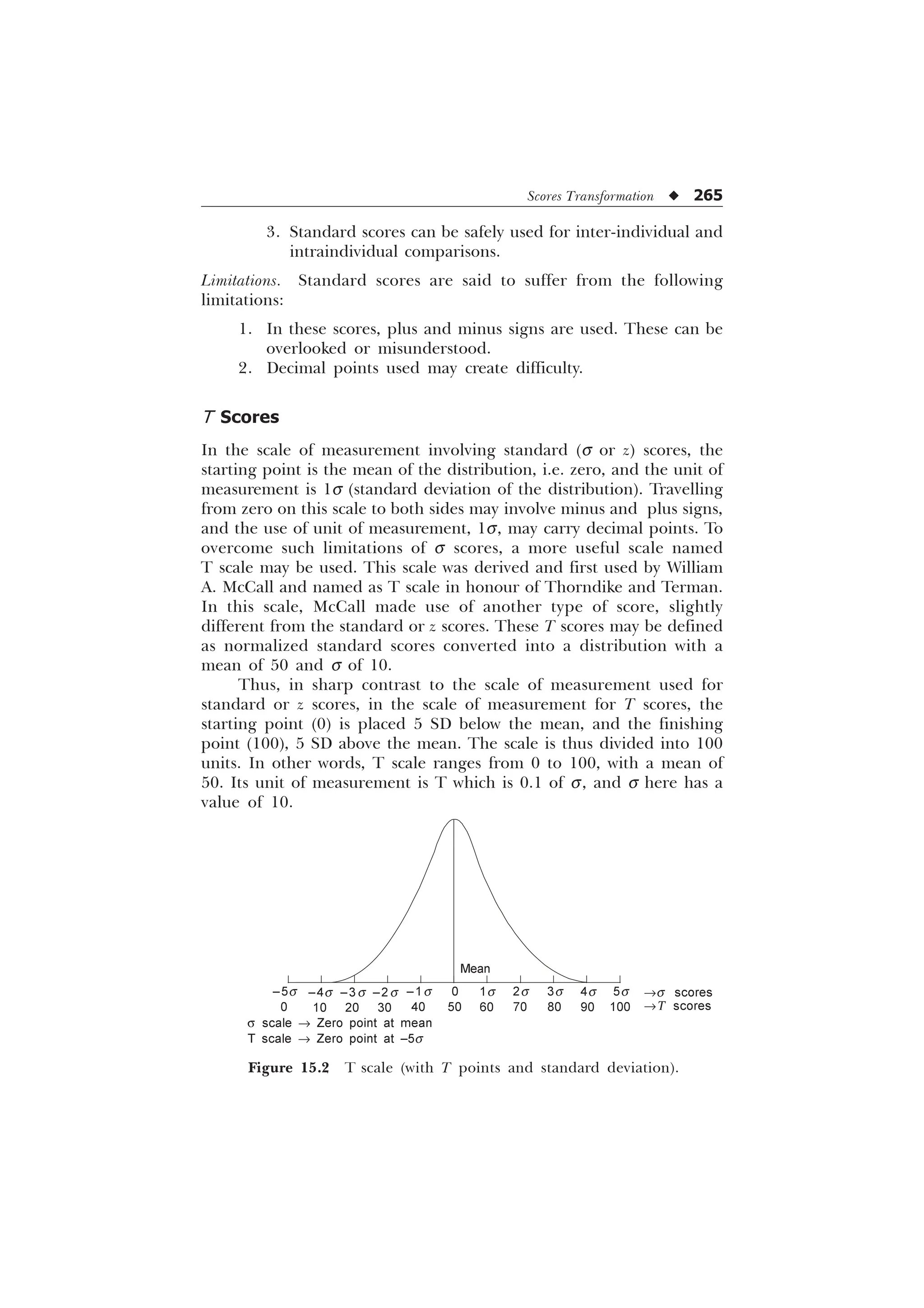
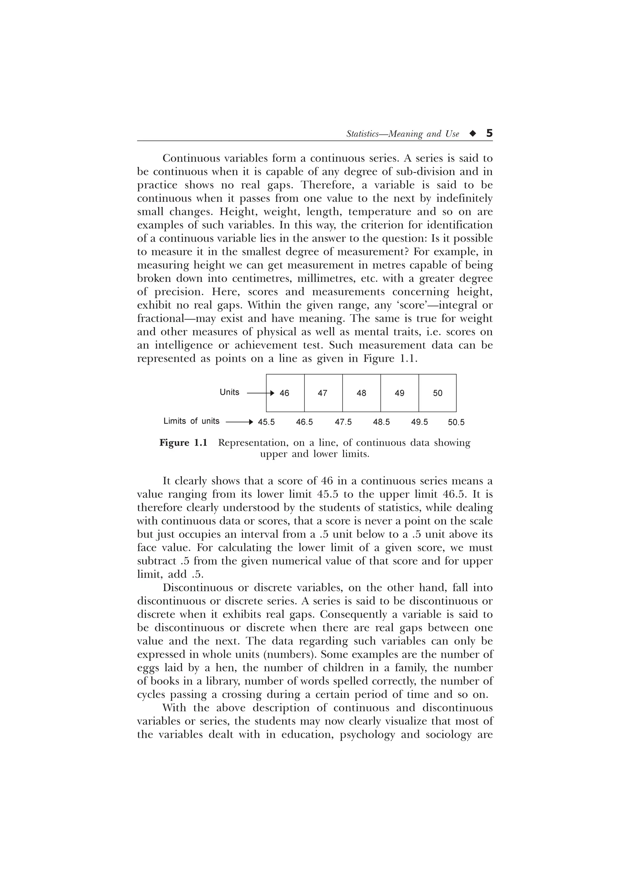
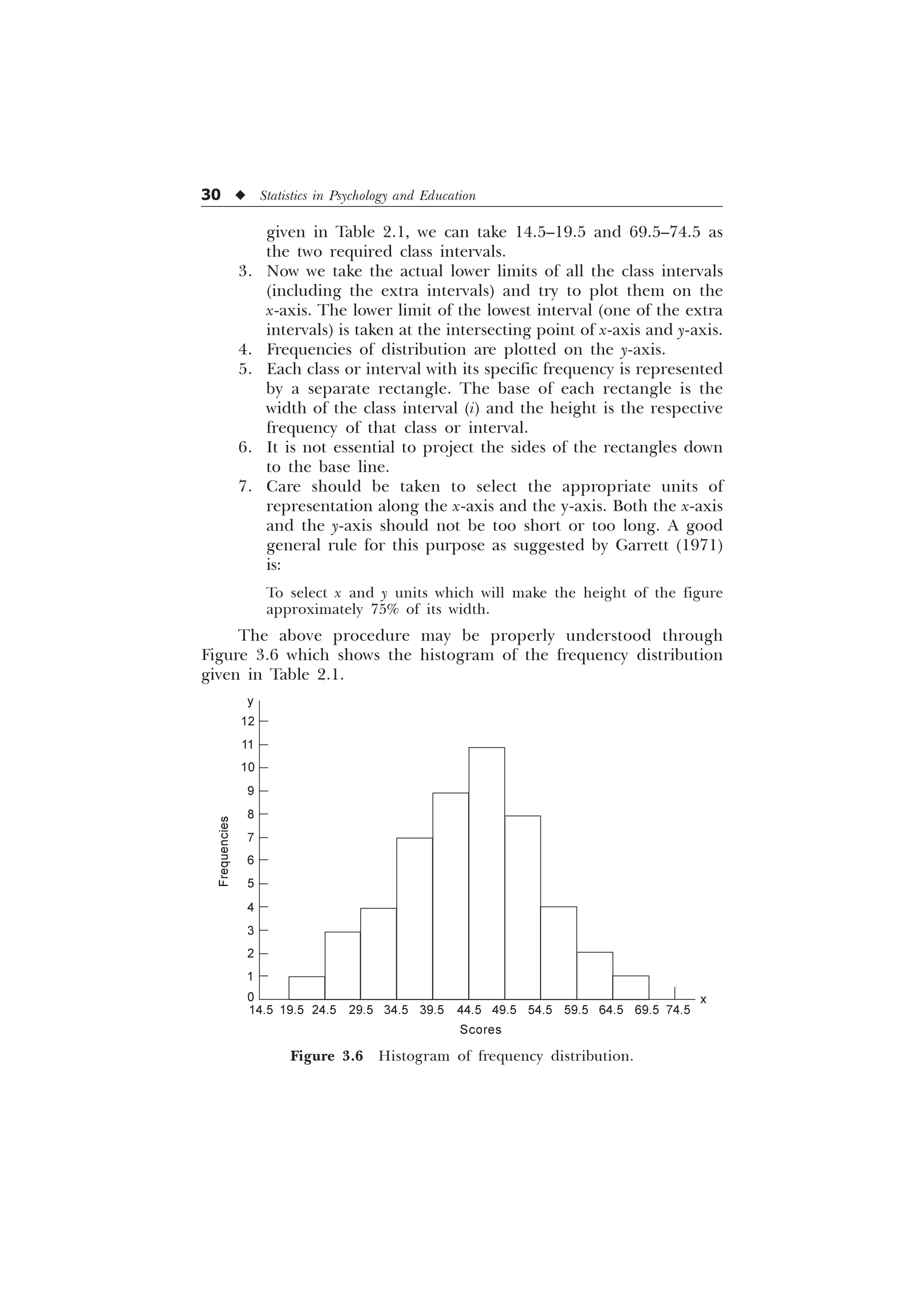
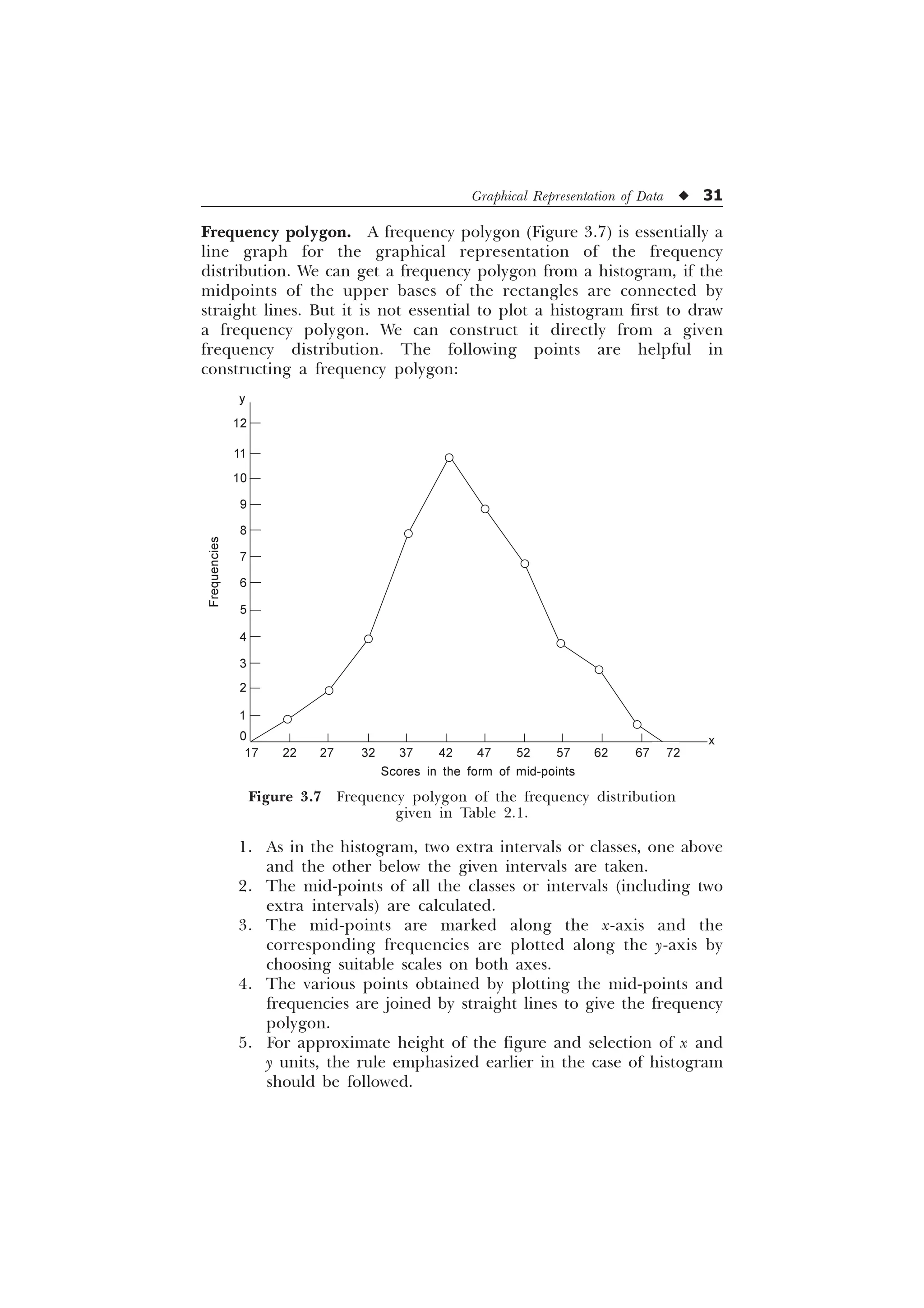
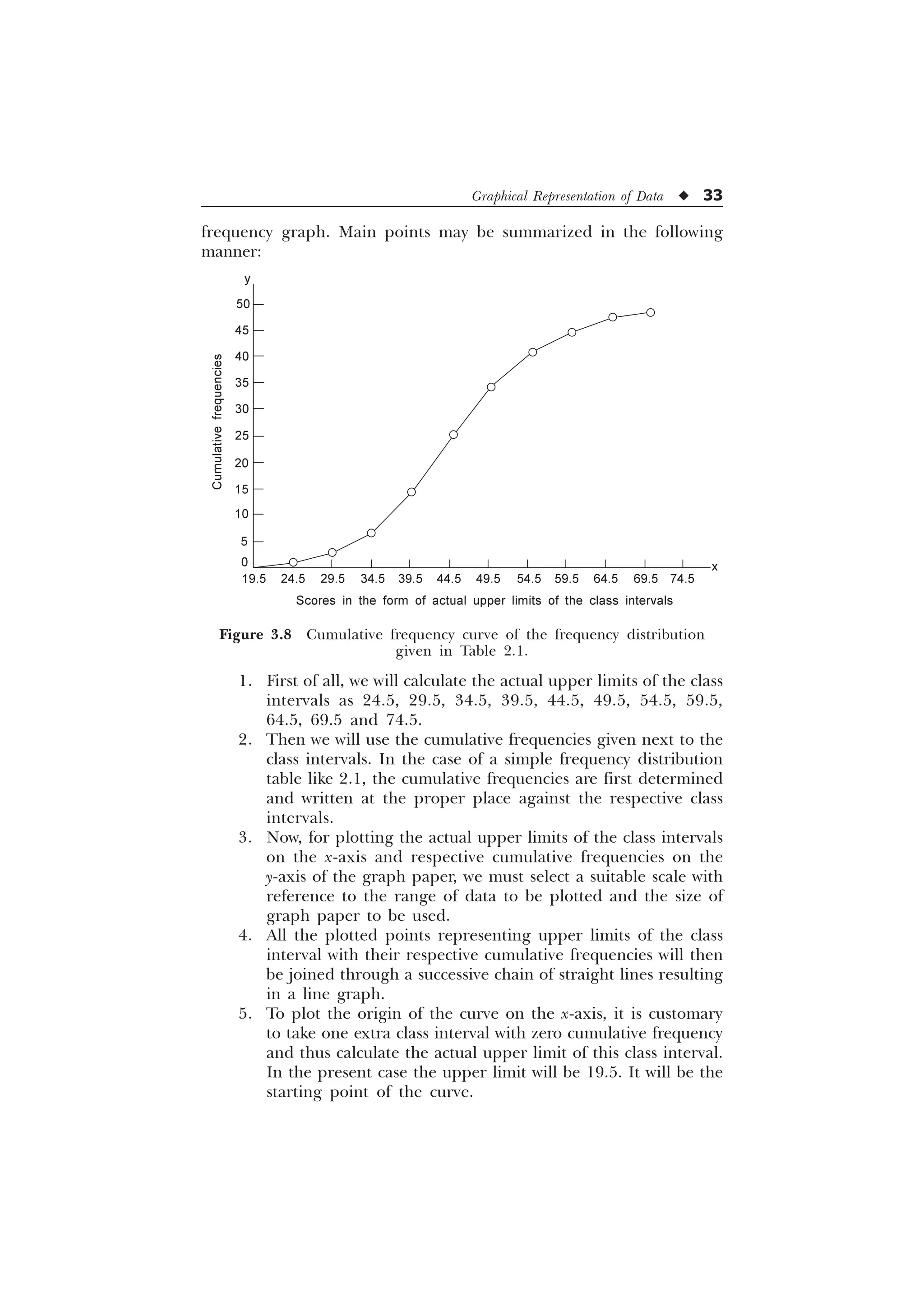
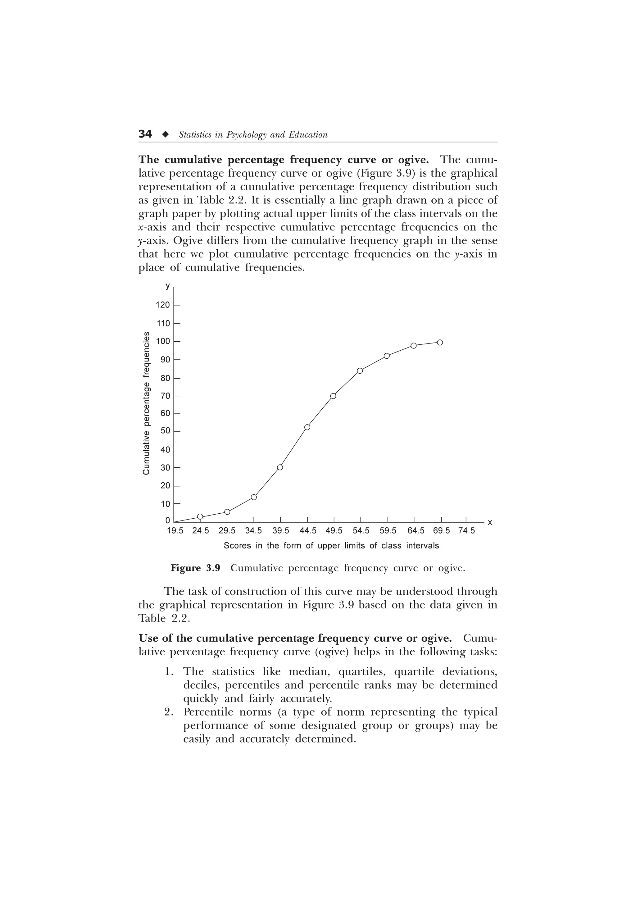
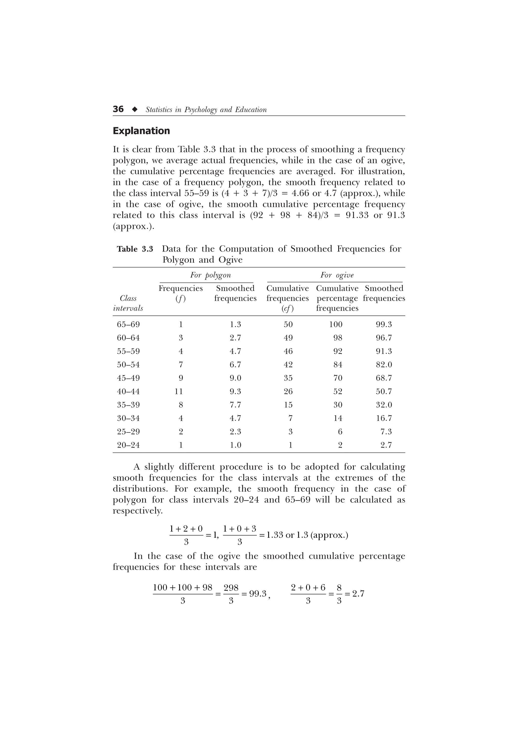
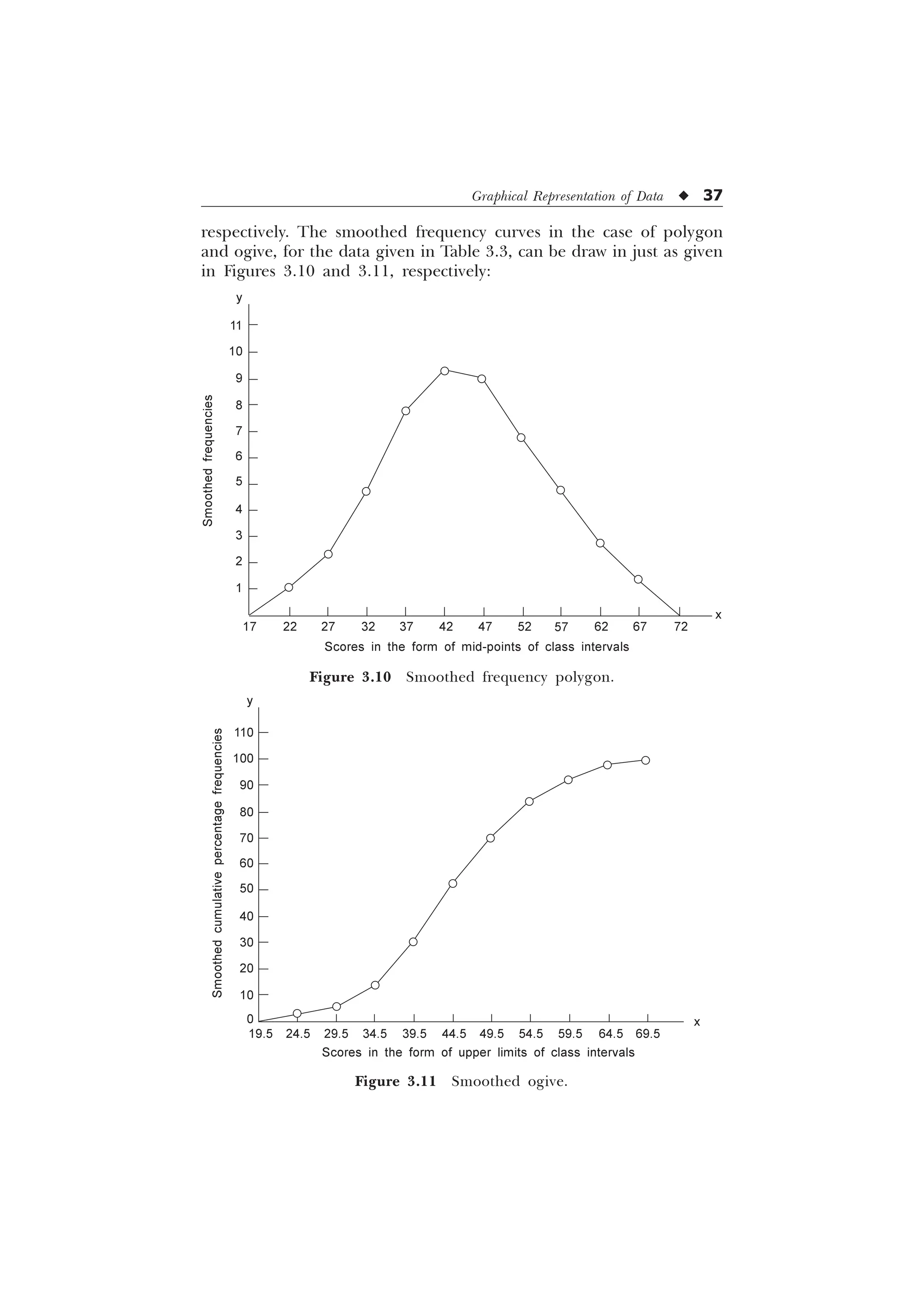
The document is a comprehensive introduction to statistics in psychology and education, authored by S.K. Mangal, and outlines both fundamental statistical concepts and advanced techniques across various chapters. It emphasizes the importance of statistical methods in evaluating and measuring in educational and psychological contexts, along with providing practical applications and exercises for learners. The second edition has been updated with new chapters and revised content to align with current academic syllabi and research areas.


![44 u Statistics in Psychology and Education
is termed as median. We may thus say that the median of a distribution
is the point on the score scale below which half (or 50%) of the scores
fall. Thus, median is the score or the value of that central item which
divides the series into two equal parts. It should therefore be
understood that the central item itself is not the median. It is only the
measure or value of the central item that is known as the median. For
example, if we arrange in ascending or descending order the marks of
5 students, then the marks obtained by the 3rd student from either
side will be termed as the median of the scores of the group of students
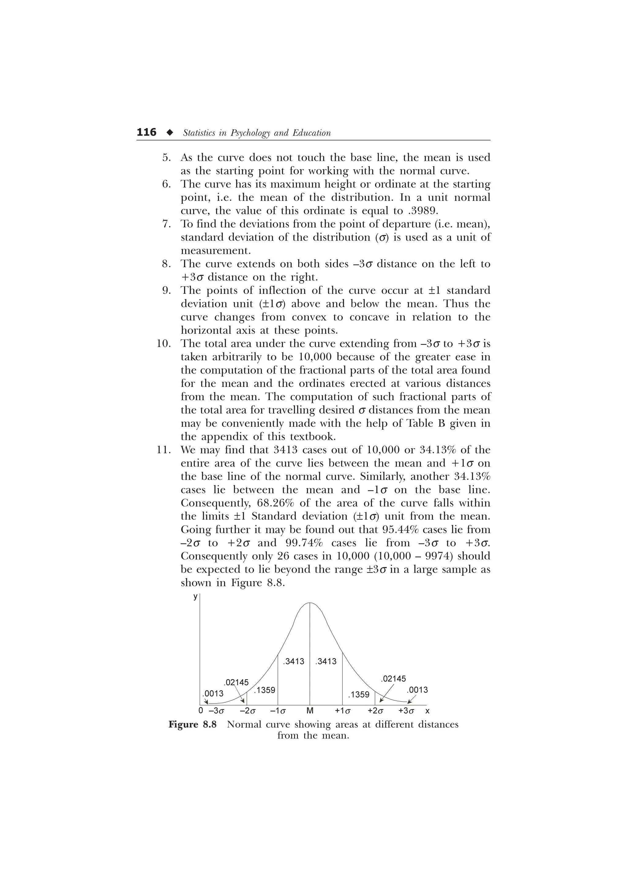
under consideration.
Computation of median for ungrouped data. The following two
situations could arise:
1. When N (No. of items in a series) is odd. In this case where N,
is odd (not divisible by 2), the median can be computed by the
formula Md = the measure or value of the (N +1)/2-th item.
Example 4.3: Let the scores obtained by 7 students on an
achievement test be 17, 47, 15, 35, 25, 39, 44. Then, first of all, for
calculating median, we have to arrange the scores in ascending or
descending order: 15, 17, 25, 35, 39, 44, 47. Here N (= 7) is odd, and
therefore, the score of the (N + 1)/2-th item or 4th student, i.e. 35
will be the median of the given scores.
2. When N (No. of items in a series) is even. In the case where N
is even (divisible by 2), the median is determined by the
following formula:
WKH YDOXH RI WK LWHP WKH YDOXH RI @WK LWHP
G
1 1
0
Example 4.4: Let there be a group of 8 students whose scores in a test
are, 17, 47, 15, 35, 25, 39, 50, 44. For calculating mean of these scores
we proceed as follows:
Arrangement of scores in ascending series: 15, 17, 25, 35, 39,
44, 47, 50
The score of the (N/2)th, i.e. 4th student = 35
The score of the [(N/2) + 1]th, i.e. 5th student = 39
Then,
Median =
= 37
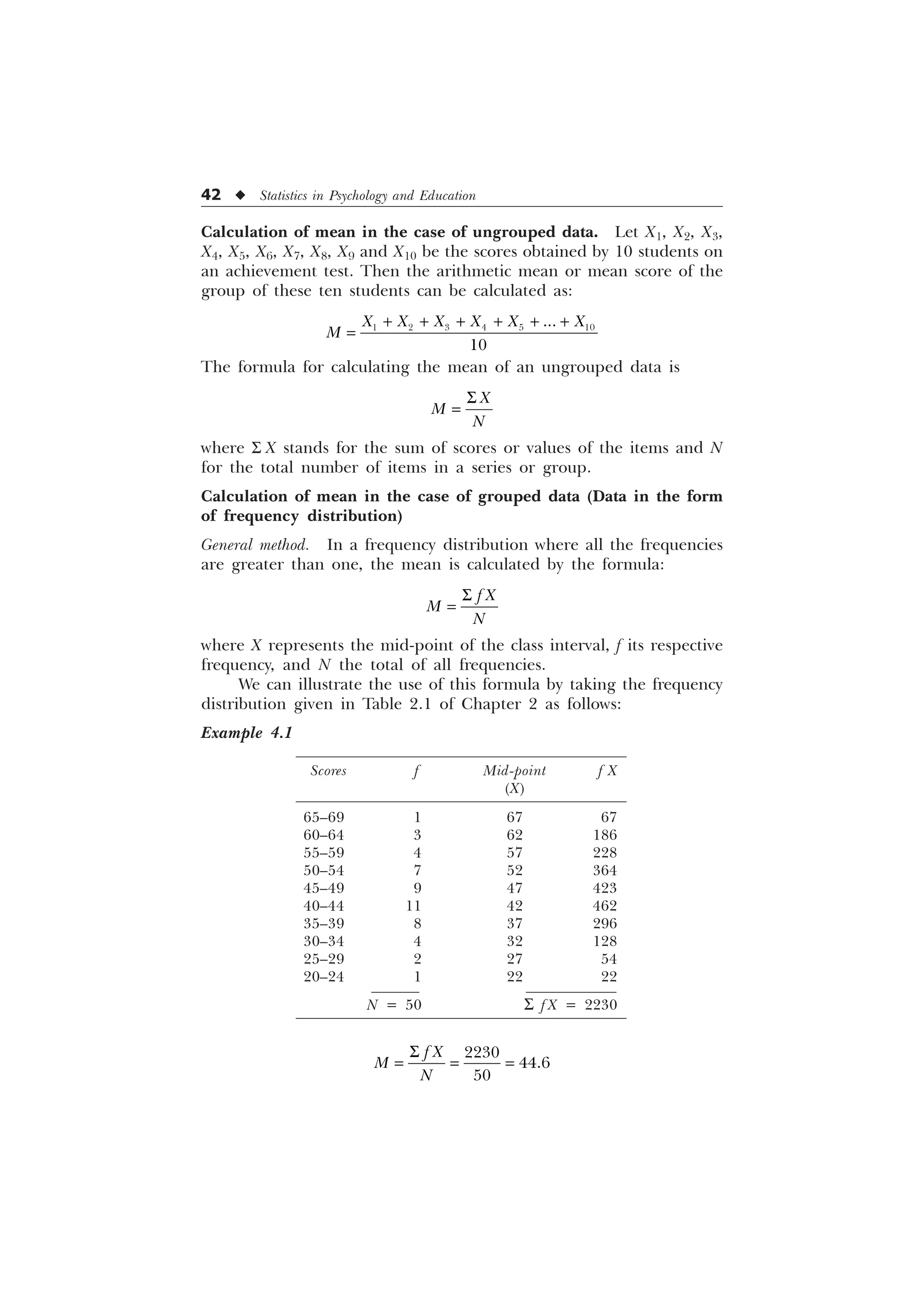
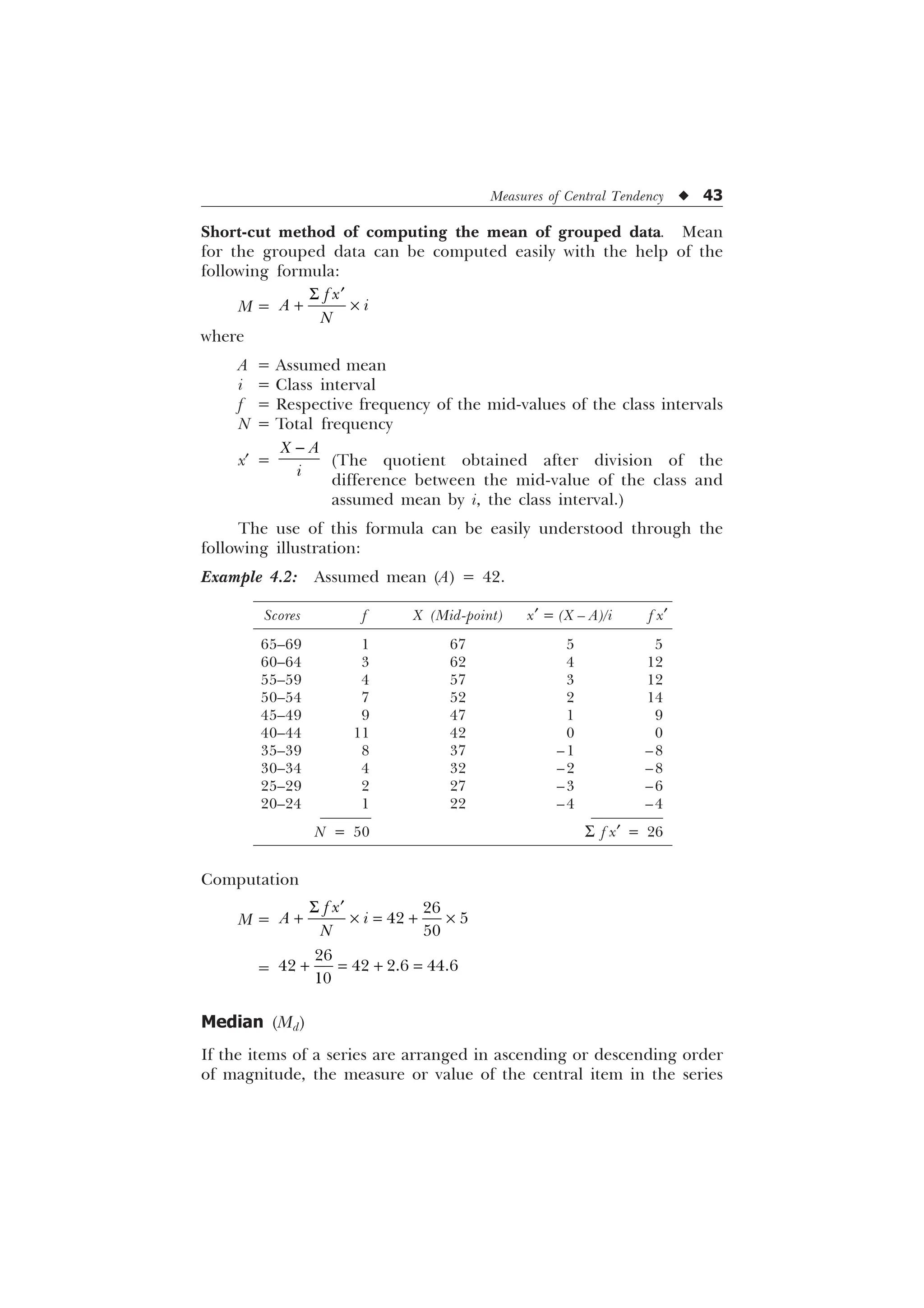
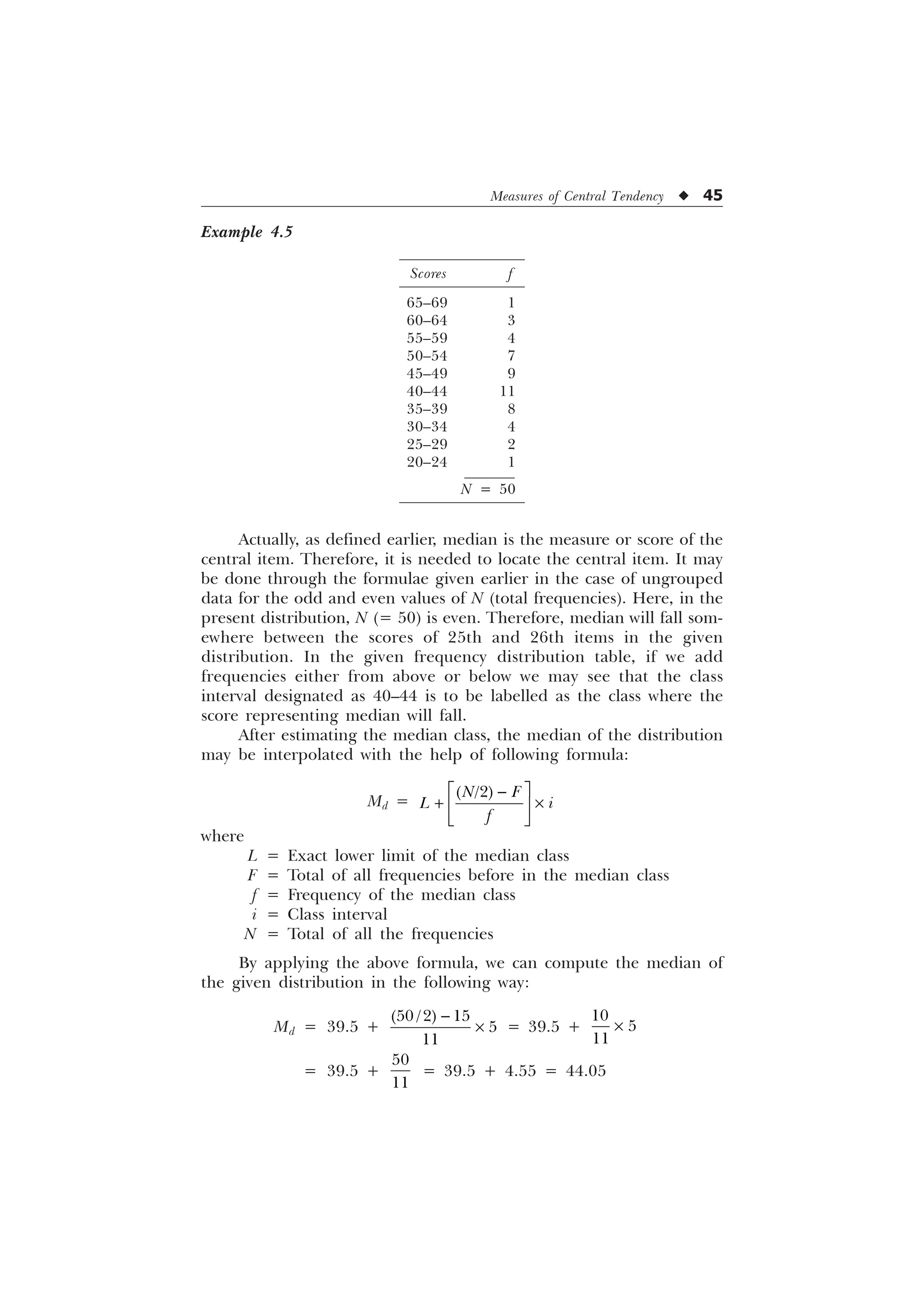
Computation of median for grouped data (in the form of frequency
distribution). If the data is available in the form of a frequency
distribution like below, then calculation of median first requires the
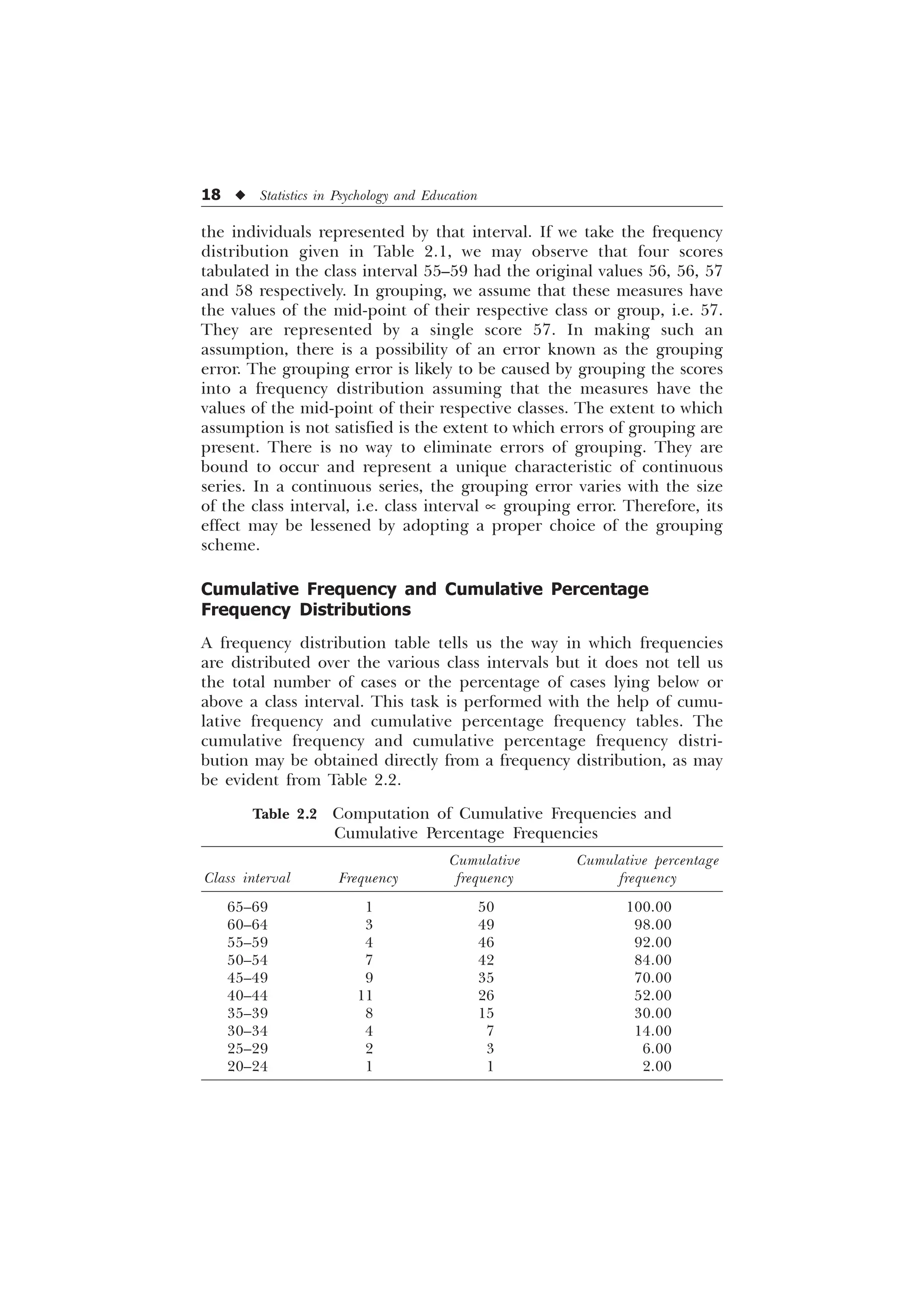
location of median class.](https://image.slidesharecdn.com/stats-s-241206101830-e3d4cc67/75/Stats-S-K-Mangal-statistics-textook-in-pdf-56-2048.jpg)
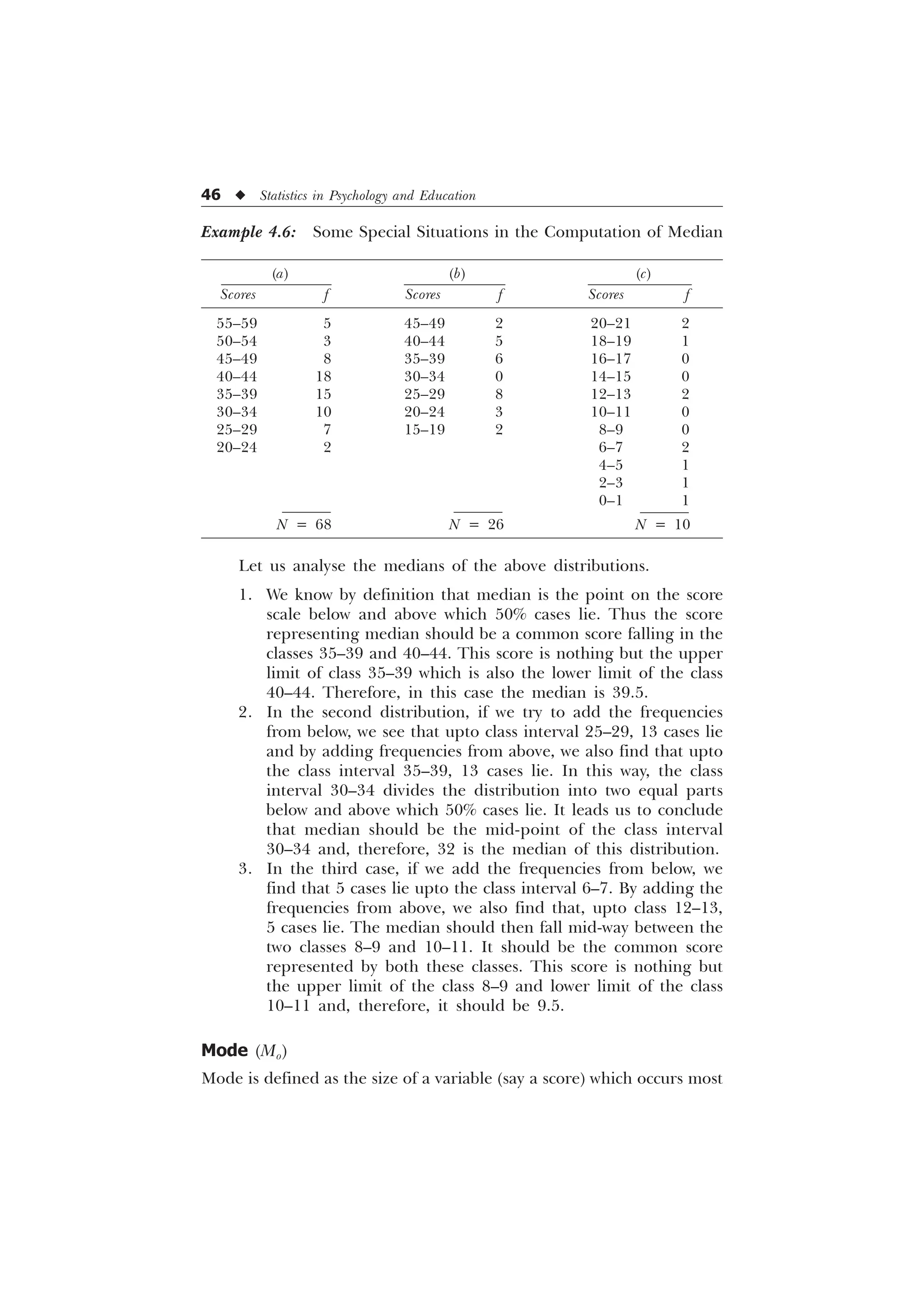
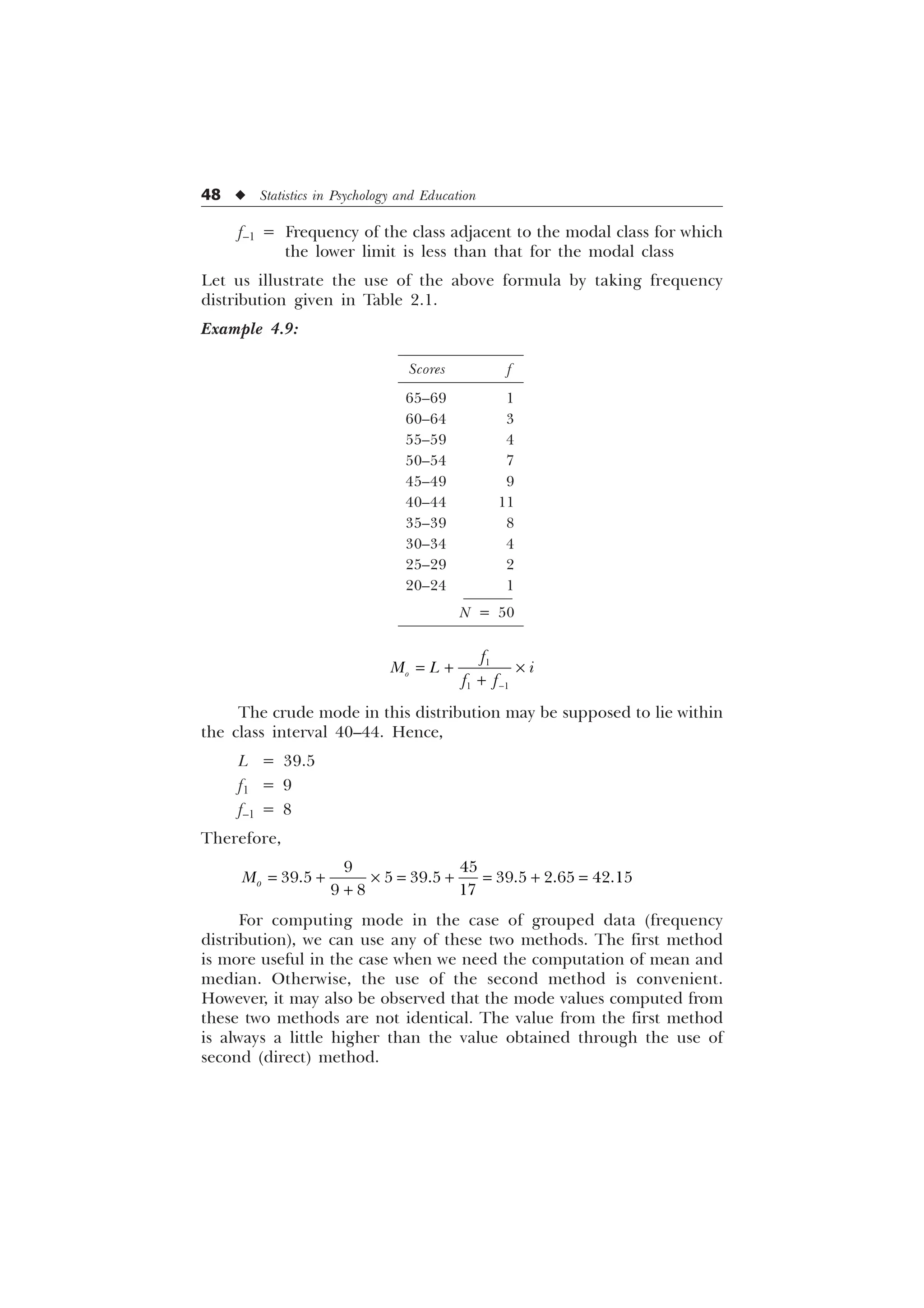
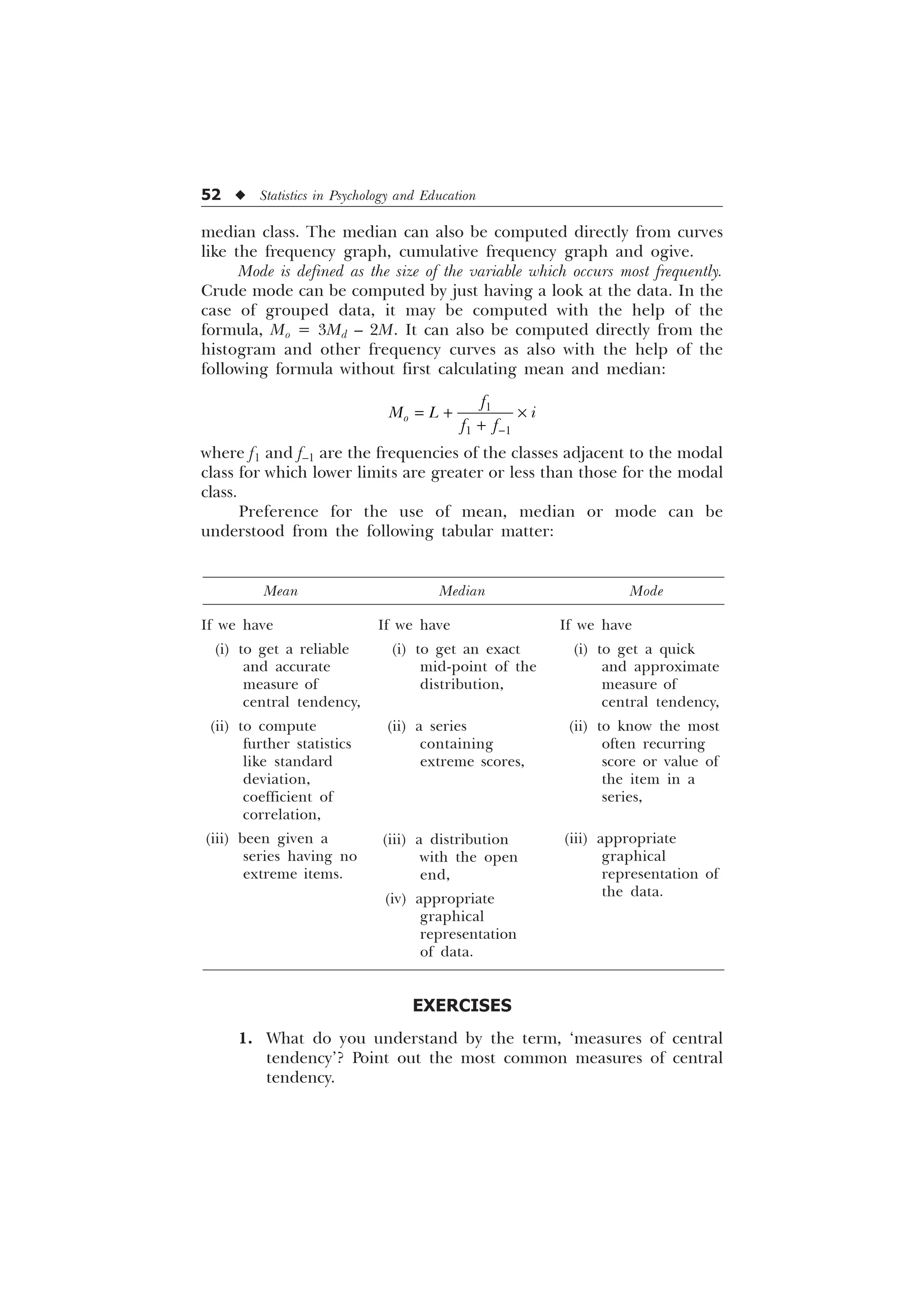
![Measures of Central Tendency u 51
2. Mode is that value of the item which occurs most frequently
or is repeated maximum number of times in a given series.
Therefore, when we need to know the most often recurring
score or value of the item in a series, we compute mode. On
account of this characteristic, mode has unique importance in
the large scale manufacturing of consumer goods. In finding
the sizes of shoes and readymade garments which fit most men
or women, the manufacturers make use of the average
indicated by mode.
3. Mode can be computed from the histogram and other
frequency curves. Therefore, when we already have a graph-
ical representation of the distribution in the form of such
figures, it is appropriate to compute mode instead of mean.
SUMMARY
The statistics, mean, median and mode, are known to be the most
common measures of central tendency. A measure of central tendency
is a sort of average or a typical value of the item in the series or some
characteristics of the members of a group. Each of these measures of
the central tendency provides a single value to represent the
characteristics of the whole group in its own way.
Mean represents the ‘average’ for an ungrouped data, the sum of
the scores divided by the total number of scores gives the value of the
mean. The mean, in the case of a grouped data is best computed with
the help of a short-cut method using the following formula:
I [
0 $ L
1
6 „
–
where A is the assumed mean,
; $
[
L
„ ,
X is the mid-point of the class interval, i the class interval, and N the
total frequencies of the distribution. Median is the score or value of
that central item which divides the series into two equal parts. Hence
when N is odd (N + 1)/2-th measure, and when N is even, the average
of (N/2)-th and [(N/2) + 1]-th item’s measure provides the value of the
median. In the case of grouped data, it is computed by the formula
–
G
1 )
0 / L
I
where L represents the lower limit of the median class, F, the total of
all frequencies before the median class, and f, the frequency of the](https://image.slidesharecdn.com/stats-s-241206101830-e3d4cc67/75/Stats-S-K-Mangal-statistics-textook-in-pdf-63-2048.jpg)
![62 u Statistics in Psychology and Education
Here, rank R of the desired score 17 is 14 and N is given as 20.
Putting these figures into the formula, we get
PR= 100 –
–
= 100 –
= 100 – 67.5 =32.5 or 32
[Ans. The percentile rank of the score 17 is 32.]
Example 5.3: In an entrance examination, a candidate ranks 35 out
of 150 candidates; find out his percentile rank.
Solution. The percentile rank is given by the formula
PR = 100 –
5
1
In this case,
R = 35 and N = 150
Hence
PR = 100 –
–
= 100 –
= 100 – 23 = 77
[Ans. Percentile rank is 77.]
From grouped data or frequency distribution
1st Method. (Direct method not needing any formula). For illus-
trating the working of this method, let us take the following
distribution (same as taken for the computation of quartiles, deciles
and percentiles) and calculate the percentile rank of the score 22.
Example 5.4
Scores f
70–79 3
60–69 2
50–59 2
40–49 3
30–39 5
20–29 4
10–19 3
0–9 2
N = 24](https://image.slidesharecdn.com/stats-s-241206101830-e3d4cc67/75/Stats-S-K-Mangal-statistics-textook-in-pdf-74-2048.jpg)
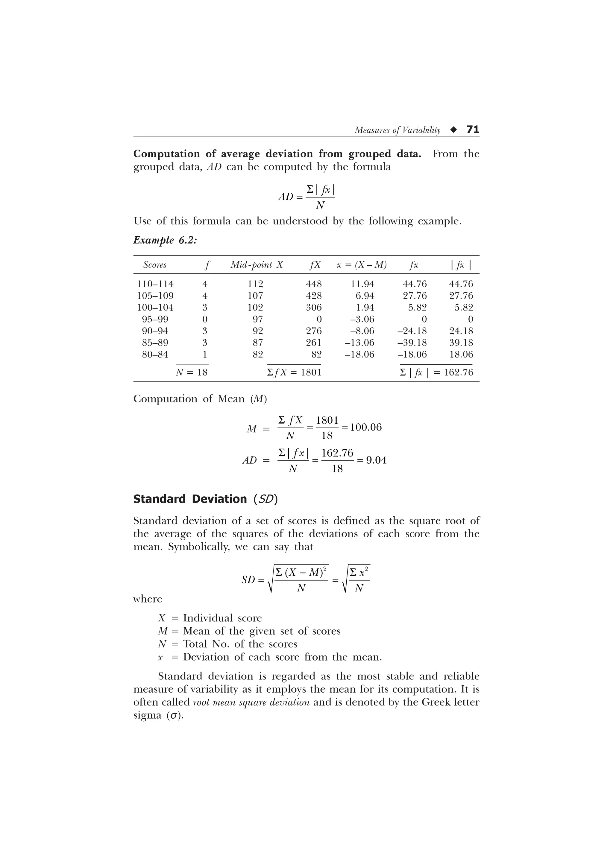
![72 u Statistics in Psychology and Education
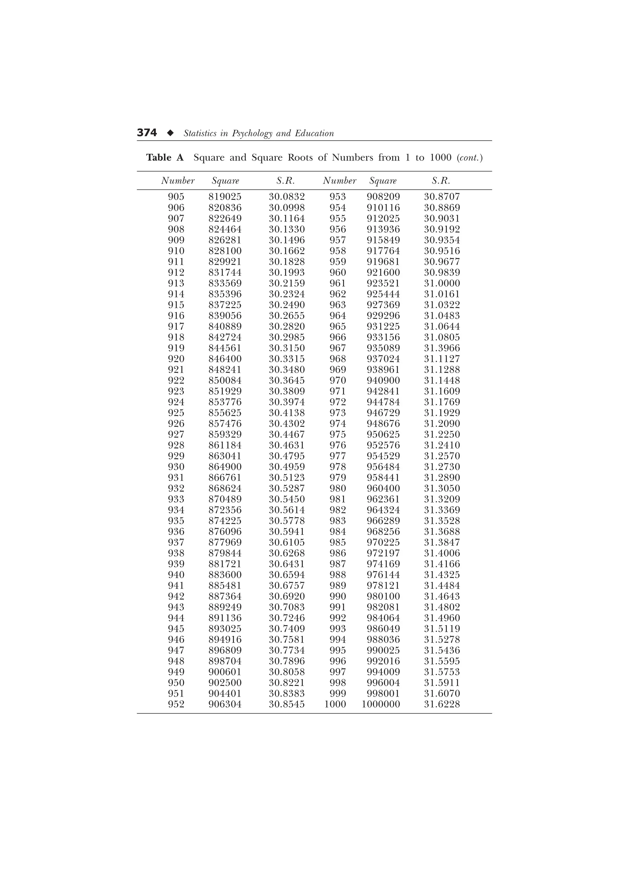
Computation of standard deviation (SD) from ungrouped data.
Standard deviation can be computed from the ungrouped scores by
the formula
T
6
[
1
The use of this formula is illustrated in the following example:
Example 6.3: Calculate SD for the following set of scores:
52, 50, 56, 68, 65, 62, 57, 70.
Solution. Mean of the given scores
M =
N = 8
Scores Deviation from the
X mean (X – M) or x x2
52 – 8 64
50 – 10 100
56 – 4 16
68 8 64
65 5 25
62 2 4
57 – 3 9
70 10 100
S x2
= 382
Formula s =
6
[
1
=
[Ans. Standard Deviation = 6.91]
Computation of SD from grouped data. Standard deviation in case
of grouped data can be computed by the formula
s =
I[
1
6
The use of the formula can be illustrated with the help of the following
example.
Example 6.4: Compute SD for the frequency distribution given below.
The mean of this distribution is 115.](https://image.slidesharecdn.com/stats-s-241206101830-e3d4cc67/75/Stats-S-K-Mangal-statistics-textook-in-pdf-84-2048.jpg)
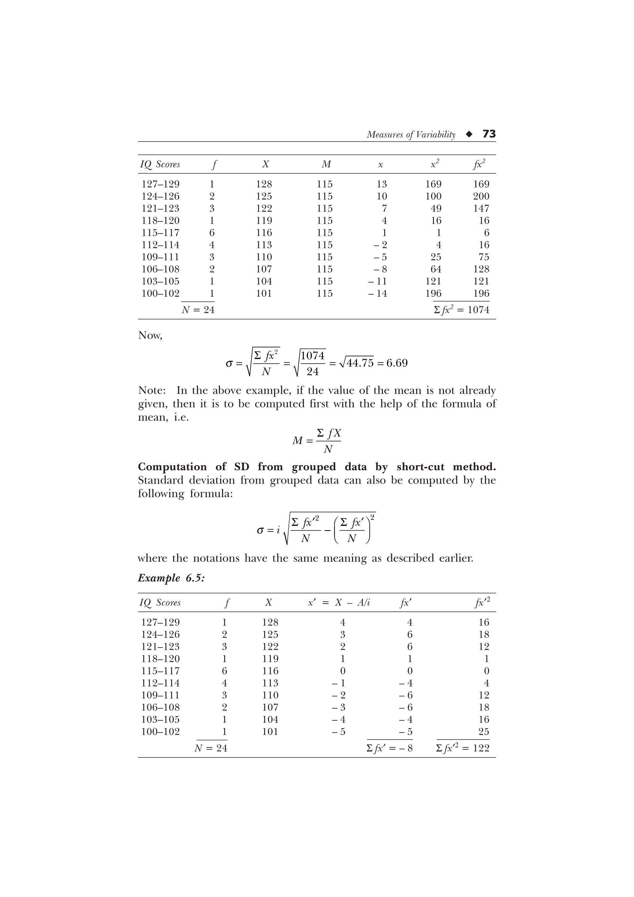
![74 u Statistics in Psychology and Education
Now putting the appropriate figures in the formula:
s =
6 6
„ „
È Ø
É Ù
Ê Ú
I[ I[
L
1 1
=
È Ø
É Ù
Ê Ú
=
–
=
–
=
= 6.69
[Ans. Standard Deviation = 6.69.]
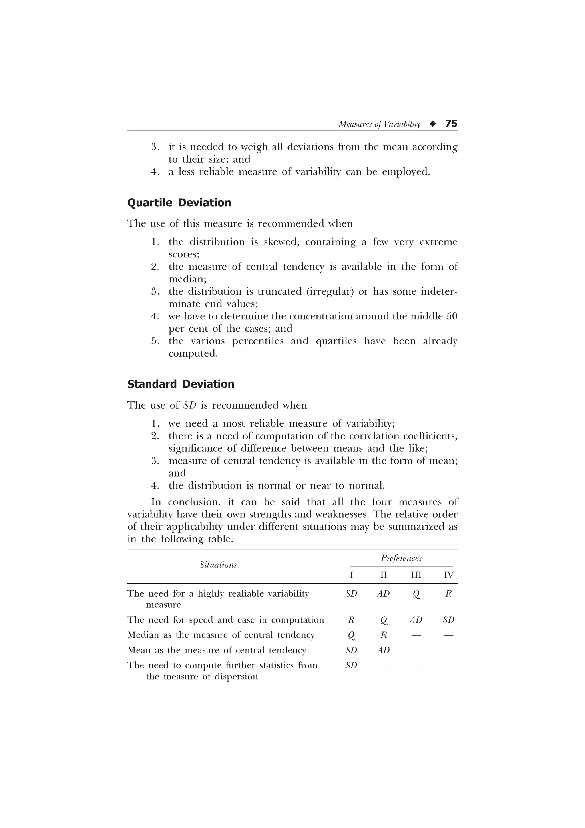
WHEN AND WHERE TO USE THE VARIOUS MEASURES OF
VARIABILITY
Range
The computation of this measure of variability is recommended when
1. we need to know simply the highest and lowest scores of the
total spread;
2. the group or distribution is too small;
3. we want to know about the variability within the group within
no time;
4. we require speed and ease in the computation of a measure of
variability; and
5. the distribution of the scores of the group is such that the
computation of other measures of variability is not much
useful.
Average Deviation
This measure is to be used when
1. distribution of the scores is normal or near to normal;
2. the standard deviation is unduly influenced by the presence of
extreme deviations;](https://image.slidesharecdn.com/stats-s-241206101830-e3d4cc67/75/Stats-S-K-Mangal-statistics-textook-in-pdf-86-2048.jpg)
![Linear Correlation u 81
17, 25, 9, 35, 18, we will rank them as 4, 2, 5, 1 and 3. We determine
the ranks or the positions of the individuals in both the given sets of
scores. These ranks are then subjected to further calculation for the
determination of the coefficient of correlation.
How is it done can be understood through the following
examples.
Example 7.1
Marks in Marks in Rank in Rank in Difference Difference
Individuals History Civics History Civics in ranks, squared
(X) (Y) (R1) (R2) irrespespective (d2
)
of
+ve or –ve signs
(R1 – R2 = |d|)
A 80 82 2 3 1 1
B 45 86 11 2 9 81
C 55 50 10 10 0 0
D 56 48 9 11 2 4
E 58 60 8 9 1 1
F 60 62 7 8 1 1
G 65 64 6 7 1 1
H 68 65 5 6 1 1
I 70 70 4 5 1 1
J 75 74 3 4 1 1
K 85 90 1 1 0 0
N = 11 S d2
= 92
r =
G
1 1
6
=
– –
–
=
= 0.58
[Ans. Rank correlation coefficient = 0.58.]](https://image.slidesharecdn.com/stats-s-241206101830-e3d4cc67/75/Stats-S-K-Mangal-statistics-textook-in-pdf-93-2048.jpg)
![82 u Statistics in Psychology and Education
Example 7.2
Scores Scores Rank in X Rank in Y |R1 – R2|
Individuals in test in test (R1) (R2) = |d|
(X) (Y) d2
A 12 21 8 6 2 4
B 15 25 6.5 3.5 3 9
C 24 35 2 2 0 0
D 20 24 4 5 1 1
E 8 16 10 9 1 1
F 15 18 6.5 8 0.5 0.25
G 20 25 4 3.5 0.5 0.25
H 20 16 4 9 5 25
I 11 16 9 9 0 0
J 26 38 1 1 0 0
N = 10 S d2
= 40.5
r =
6
G
1 1
=
–
=
–
–
=
= 0.755
[Ans. Rank correlation coefficient = 0.755.]
Steps for the calculation of r:
Step 1. First, a position or a rank is assigned to each individual on
both the tests. These ranks are put under column 3 (designated R1)
and column 4 (designated R2), respectively. The task of assigning ranks,
as in Example 1, is not difficult. But as in Example 2, where two or
more individuals are found to have achieved the same score, some
difficulty arises. In this example, in the first test, X, B and F are two
individuals who have the same score, i.e. 15. Therefore, score 15
occupies the 6th position in order of merit. But now the question arises
as to which one of the two individuals B and F should be ranked 6th
or 7th. In order to overcome this difficulty we share the 6th and 7th
rank equally between them and thus rank each one of them as 6.5.
Similarly, if there are three persons who have the same score and
share the same rank, we take the average of the ranks claimed by these
persons. For example, we can take score 20 in Example 2 which is](https://image.slidesharecdn.com/stats-s-241206101830-e3d4cc67/75/Stats-S-K-Mangal-statistics-textook-in-pdf-94-2048.jpg)
![Linear Correlation u 85
Substituting these values of sx and sy in (i) we get
r =
6 6
6 6 6 6
[ [
[ [
1
1 1
(ii)
The use of this formula may be illustrated through the following
example:
Example 7.3
Individuals Scores in test Scores in test
X Y x y xy x2
y2
A 15 60 –10 10 –100 100 100
B 25 70 0 20 0 0 400
C 20 40 –5 –10 50 25 100
D 30 50 5 0 0 25 0
E 35 30 10 –20 –200 100 400
S xy S x2
S y2
= – 250 = 250 = 1000
Mean of series X, MX = 25
Mean of series Y, MY = 50
r =
6
–
6 6
[
[
=
=
1
0.5
2
[Ans. Product moment correlation coefficient = –0.5.]
Computation of r directly from raw scores when deviations are taken from zero
(without calculating deviation from the means). In this case, product
moment r is to be computed by the following formula:
6 6 6
Ë Û Ë Û
6 6 6 6
Í Ý Í Ý
1 ; ;
U
1 ; ; 1](https://image.slidesharecdn.com/stats-s-241206101830-e3d4cc67/75/Stats-S-K-Mangal-statistics-textook-in-pdf-97-2048.jpg)
![86 u Statistics in Psychology and Education
where
X and Y = Raw scores in the test X and Y.
XY = Sum of the products of each X score multiplied with
its corresponding Y score
N = Total No. of cases or scores
The use of this formula may be understood through the following
example:
Example 7.4
Scores in Scores in
Subject test X test Y XY X2
Y2
A 5 12 60 25 144
B 3 15 45 9 225
C 2 11 22 4 121
D 8 10 80 64 100
E 6 18 108 36 324
N = 5 S X = 24 S Y = 66 S XY = 315 S X2
= 138 S Y2
= 914
r =
6 6 6
Ë Û Ë Û
6 6 6 6
Í Ý Í Ý
1 ; ;
1 ; ; 1
Here,
r =
– –
– – –
=
=
–
=
[Ans. Product moment correlation coefficient = –0.48.]
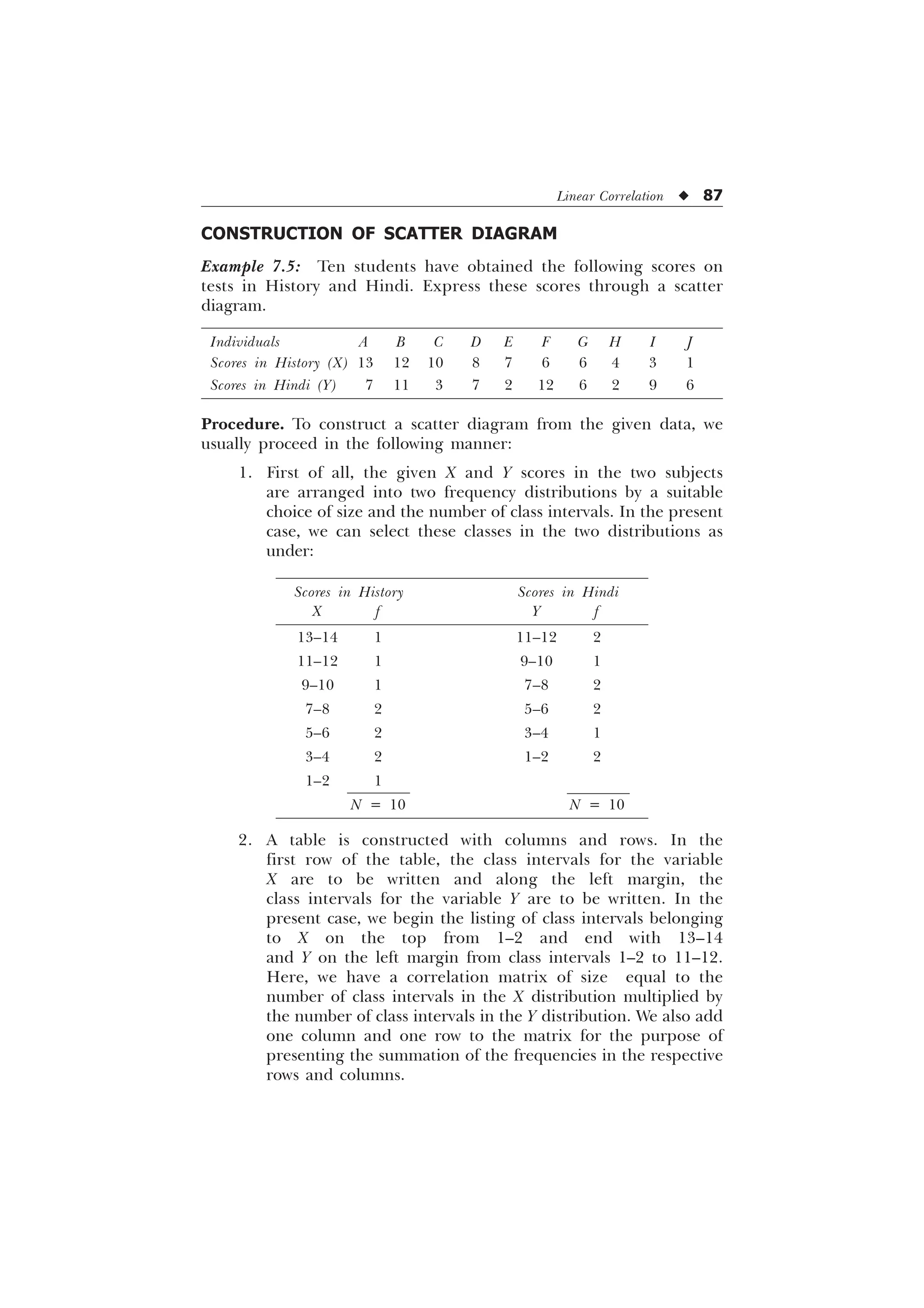
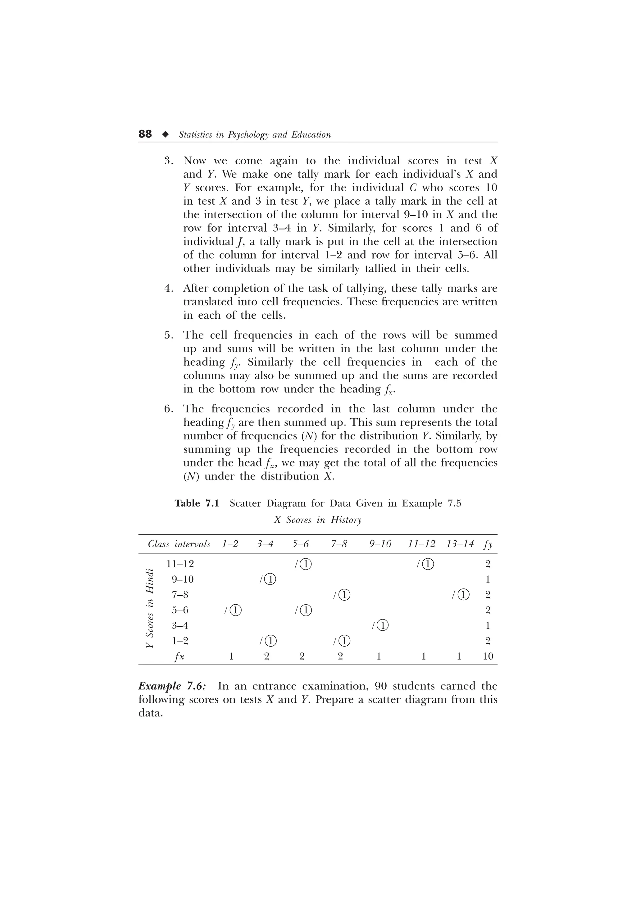
Computation of product moment r with the help of a scatter diagram or
correlation table. Product moment r may be computed through a scatter
diagram or correlation table. If this diagram or table is not given, then
the need of its construction arises. Let us illustrate the construction of
a scatter diagram or a correlation table with the help of some hypo-
thetical data.](https://image.slidesharecdn.com/stats-s-241206101830-e3d4cc67/75/Stats-S-K-Mangal-statistics-textook-in-pdf-98-2048.jpg)
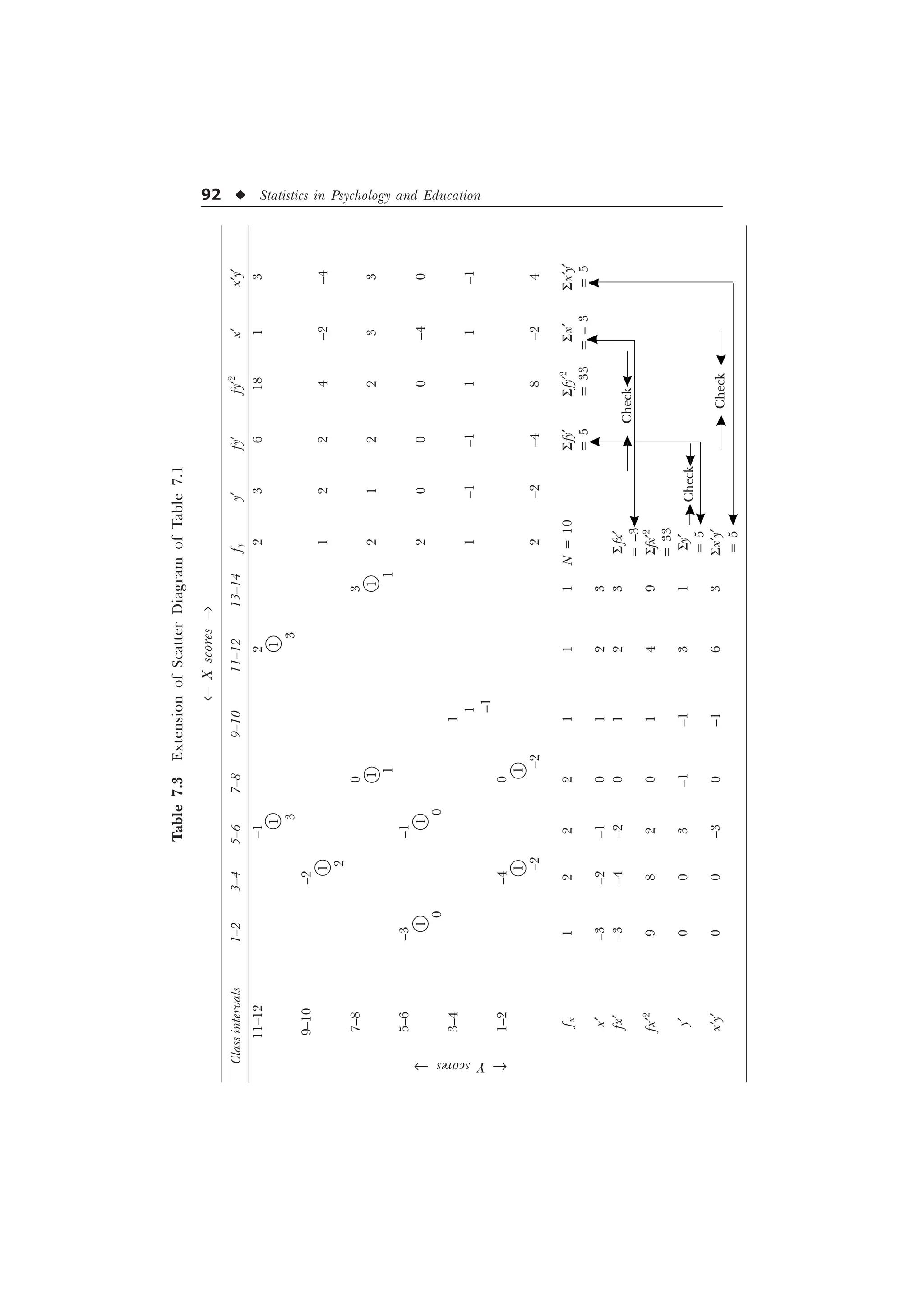
![Linear Correlation u 91
Computation of r
We know that the gereral formula for computing r is
T T
6
[
[
U
1
Here x and y denote the deviations of X and Y scores from their
respective means. When we take deviations from the assumed means of
the two distributions, this formula is likely to be changed to the one
below:
r =
6 6 6
„ „ „ „
Ë Û Ë Û
6 6 6 6
„ „ „ „
Í Ý Í Ý
1 [ I [ I
1 I [ I [ 1 I I
It may be observed that in computing r by the above formula, we need
to know the values of S x¢ y¢, S fx¢, S fy¢, S fx¢2
and S fy¢2
. All these values
may be conveniently computed through a scatter diagram. The process
of determining these is illustrated through the extension of scatter
diagrams constructed in Tables 7.1 and 7.2.
Now just look into the Table 7.3, here we can get the values
S x¢ y¢ = 5, S fx¢ = –3, S fy¢ = 5
S fx¢2
= 33, S fy¢2
= 33
Putting these values in the formula for computing r, we get
r =
–
– –
Ë ÛË Û
Í ÝÍ Ý
=
Ë Û
Ë Û
Í Ý
Í Ý
=
–
=
=
= 0.207
= 0.21 (approx.)
[Ans. Product moment coefficient of correlation = 0.21.]](https://image.slidesharecdn.com/stats-s-241206101830-e3d4cc67/75/Stats-S-K-Mangal-statistics-textook-in-pdf-103-2048.jpg)
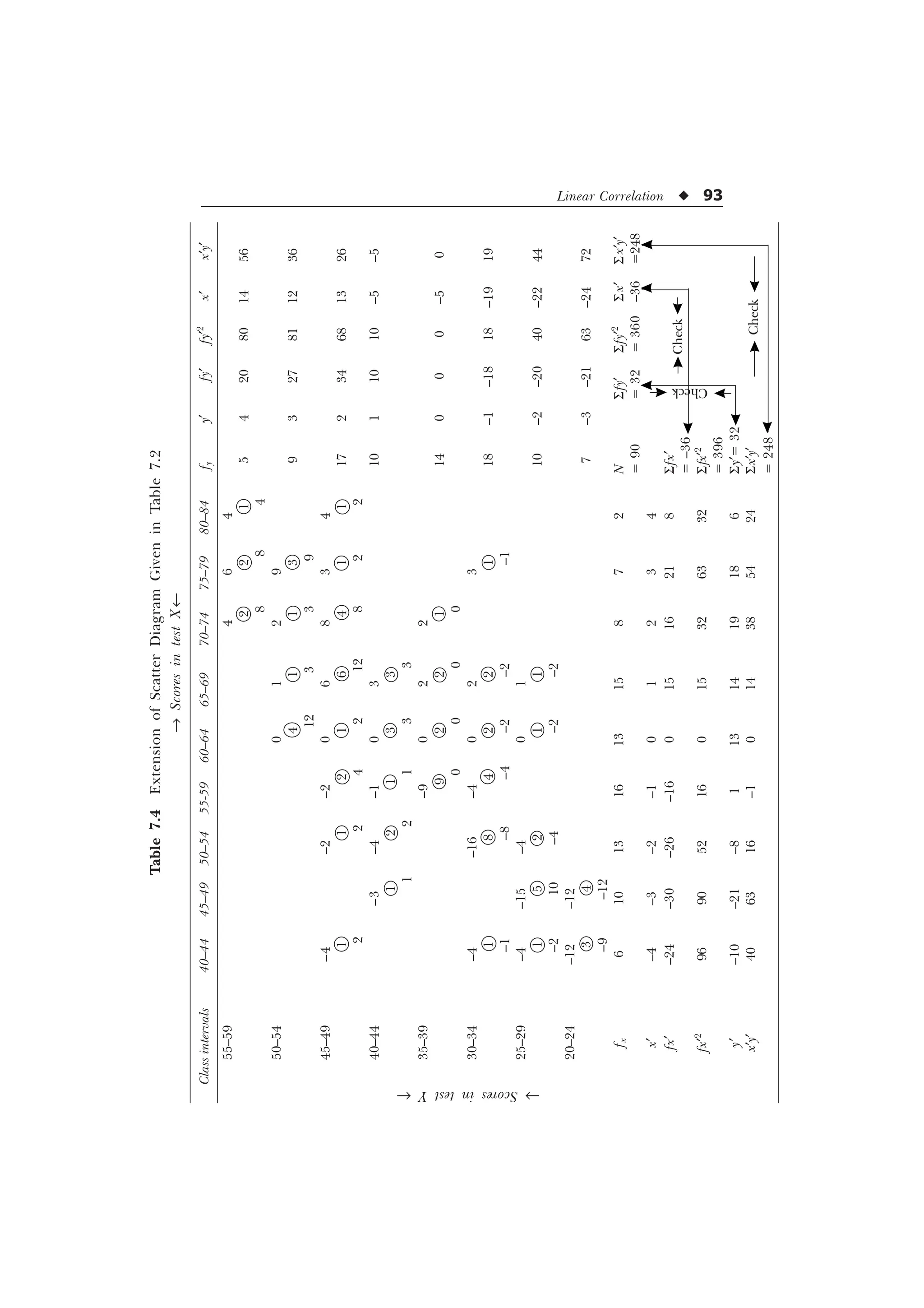
![94 u Statistics in Psychology and Education
Now putting the relevant values in the formula, we get
r =
6 6 6
„ „ „ „
Ë Û Ë Û
6 6 6 6
„ „ „ „
Í Ý Í Ý
1 [ I [ I
1 I [ I [ 1 I I
=
– –
Ë ÛË Û
– – – –
Í ÝÍ Ý
=
=
–
=
=
= 0.715 = 0.73 (approx).
[Ans. Pearson’s correlation coefficient = 0.73]
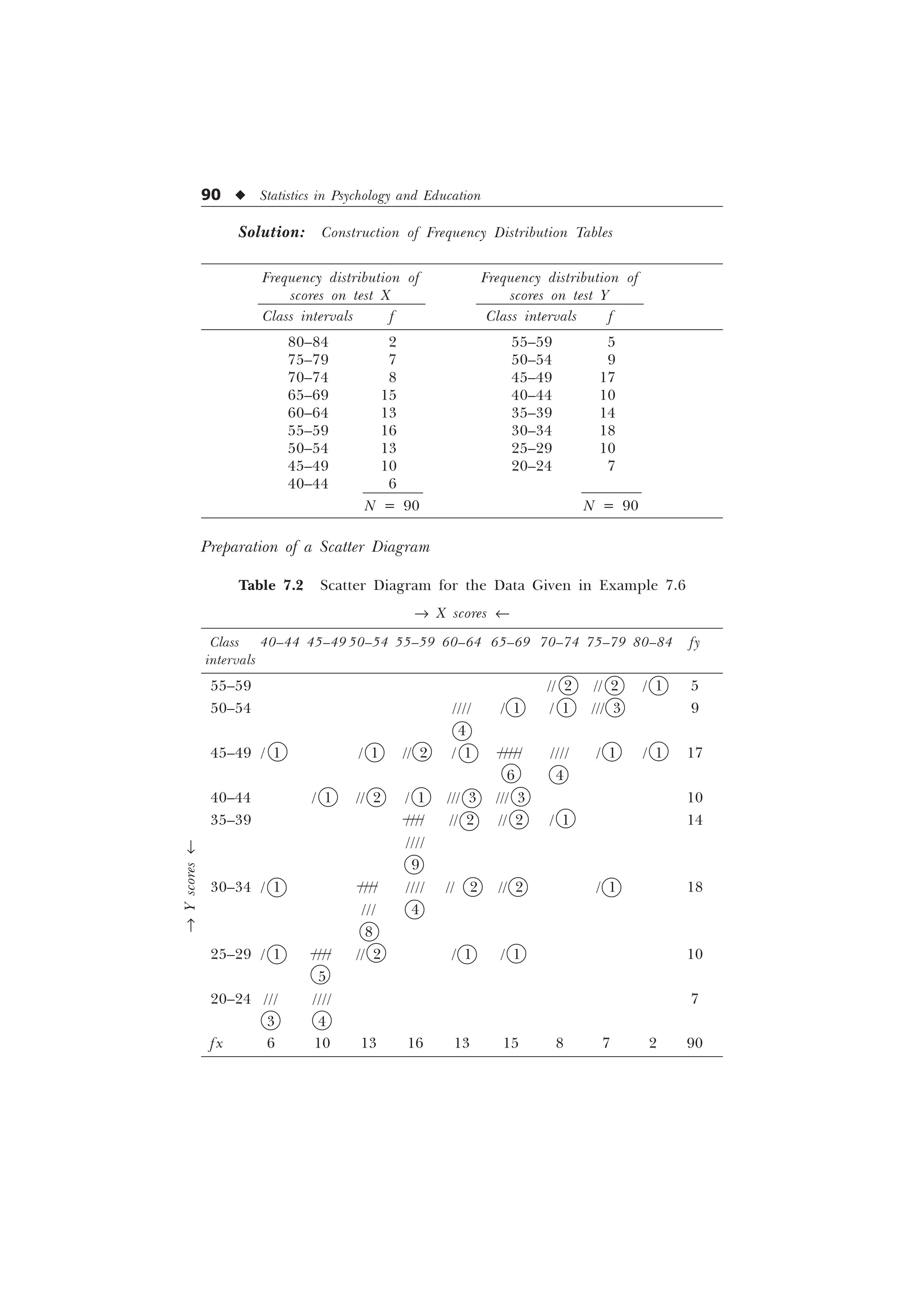
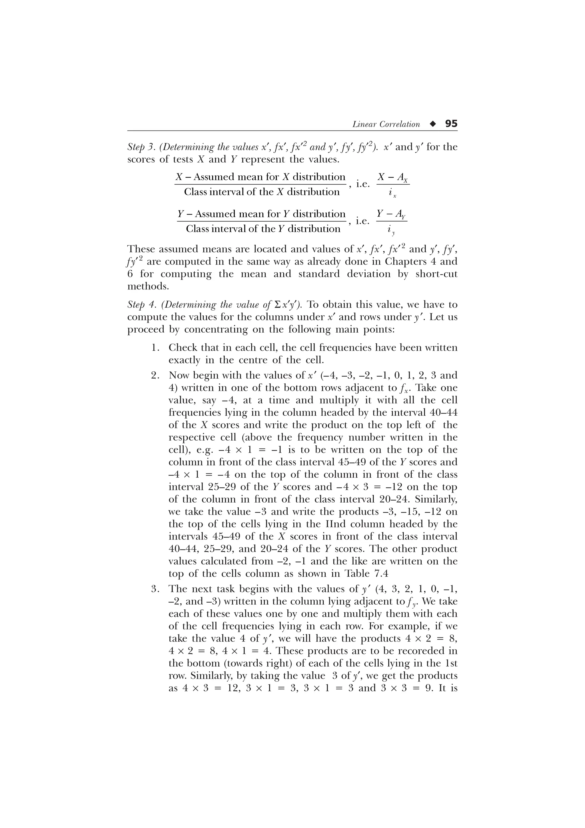
Explanation of the process of computation of r from scatter
diagrams. Let us consider the process of the computation of the
values of S fx, S fy, S fx¢2
, S fy¢2
and S x¢y¢ with the help of the scatter
diagram computed above in Tables 7.3 and 7.4 and then the
determination of r from the formula. The various steps involved are
as follows:
Step 1. (Completion of the scatter diagram). The scatter diagram in its
complete form must have one row and one column designated fx and
fy respectively for the total of the frequencies belonging to each class
interval of the scores in test X and Y. If the totals are not given (in the
assigned scatter diagram) then they are to be computed and written in
the row and column headed by fx and fy. The grand total of these rows
and columns should tally with each other. There grand totals were 10
and 90 respectively in our problem.
Step 2. (Extension of the scatter diagram). The scatter diagram is now
extended by 5 columns designated y¢, f y¢, fy¢2
, x¢ and x¢y¢ and 5 rows
designated x¢, fx¢, fx¢2
, y¢, and x¢y¢. At the end of each of these columns
and rows, the provision for the sum (S values) is also to be kept.](https://image.slidesharecdn.com/stats-s-241206101830-e3d4cc67/75/Stats-S-K-Mangal-statistics-textook-in-pdf-106-2048.jpg)
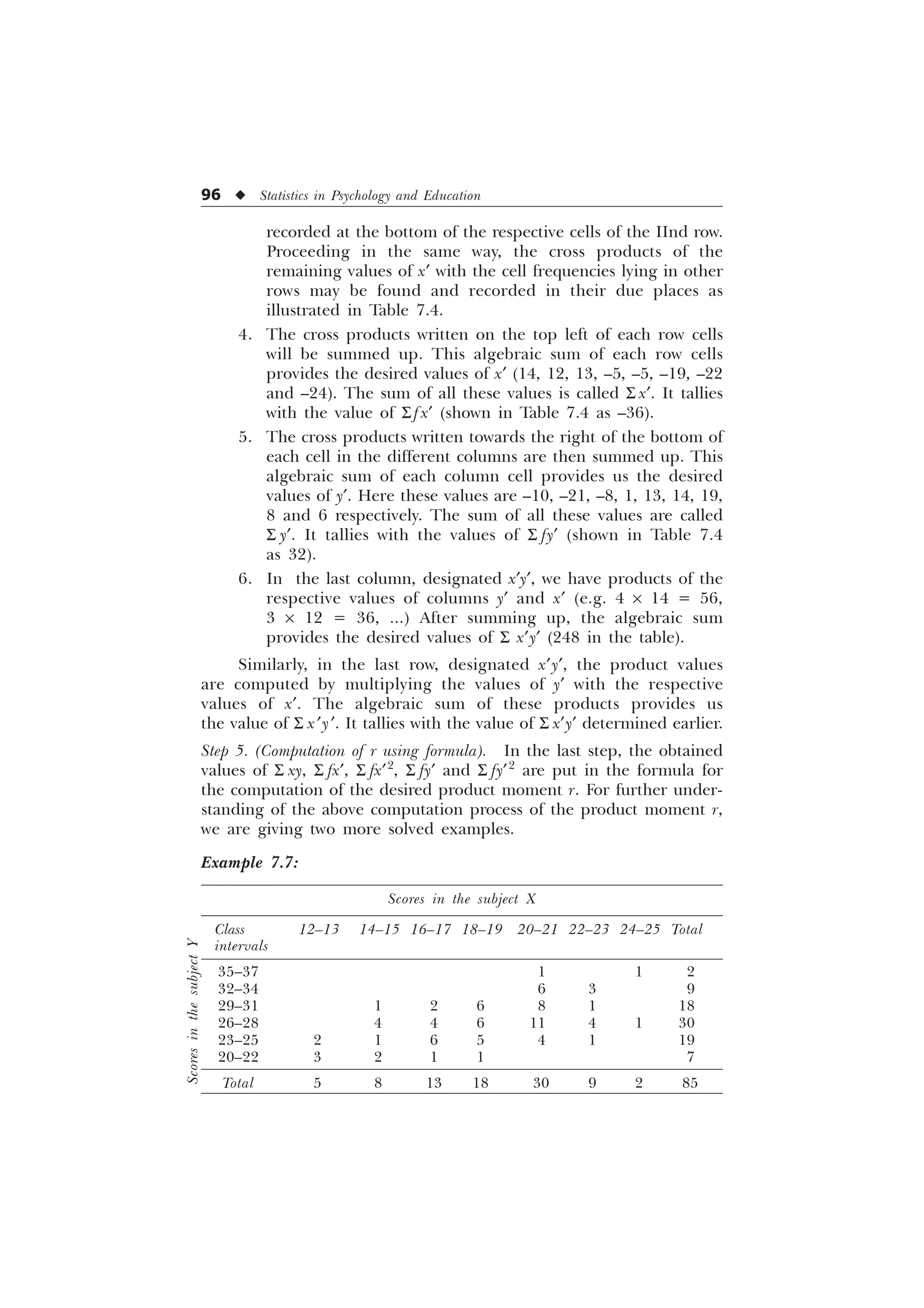
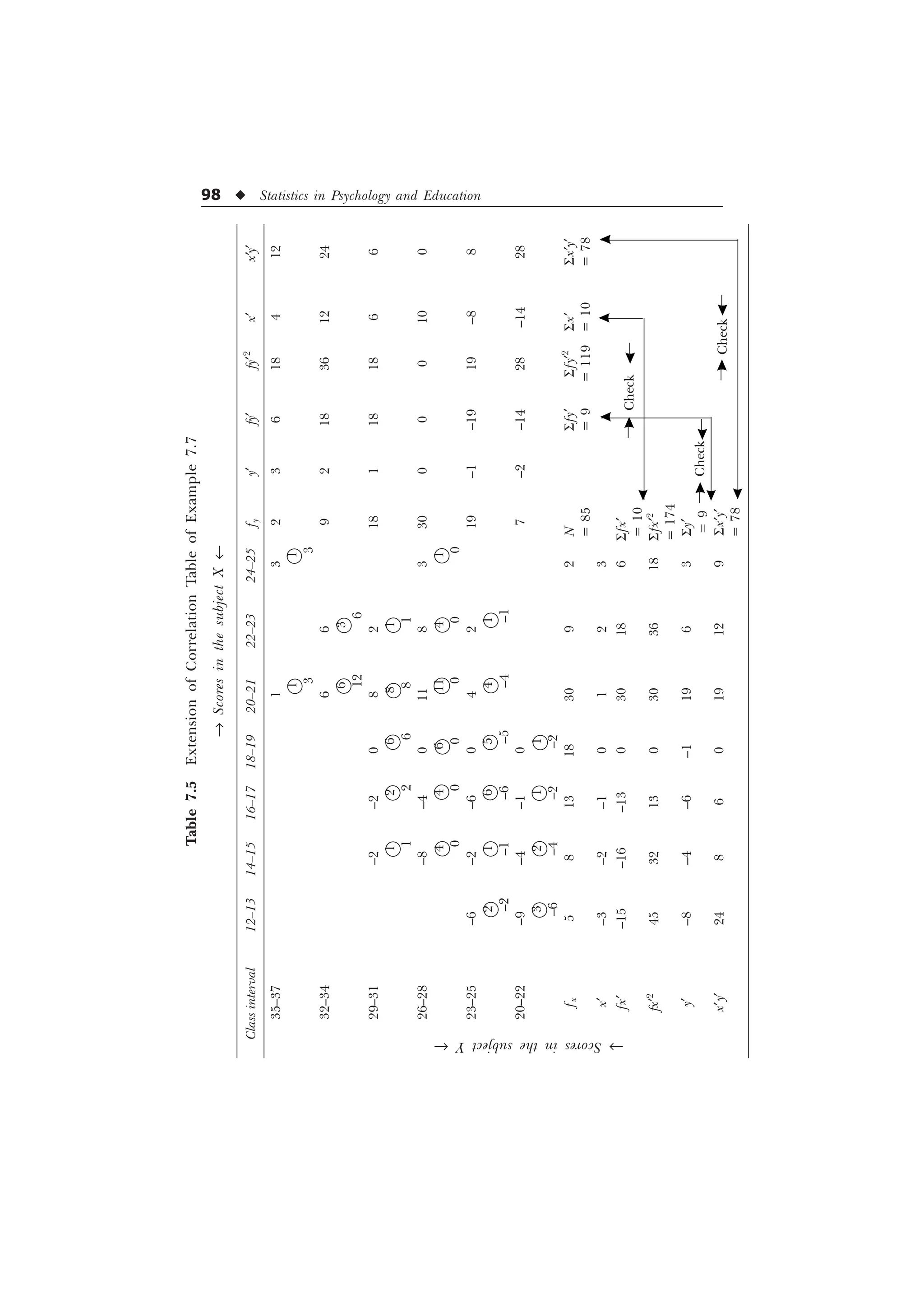
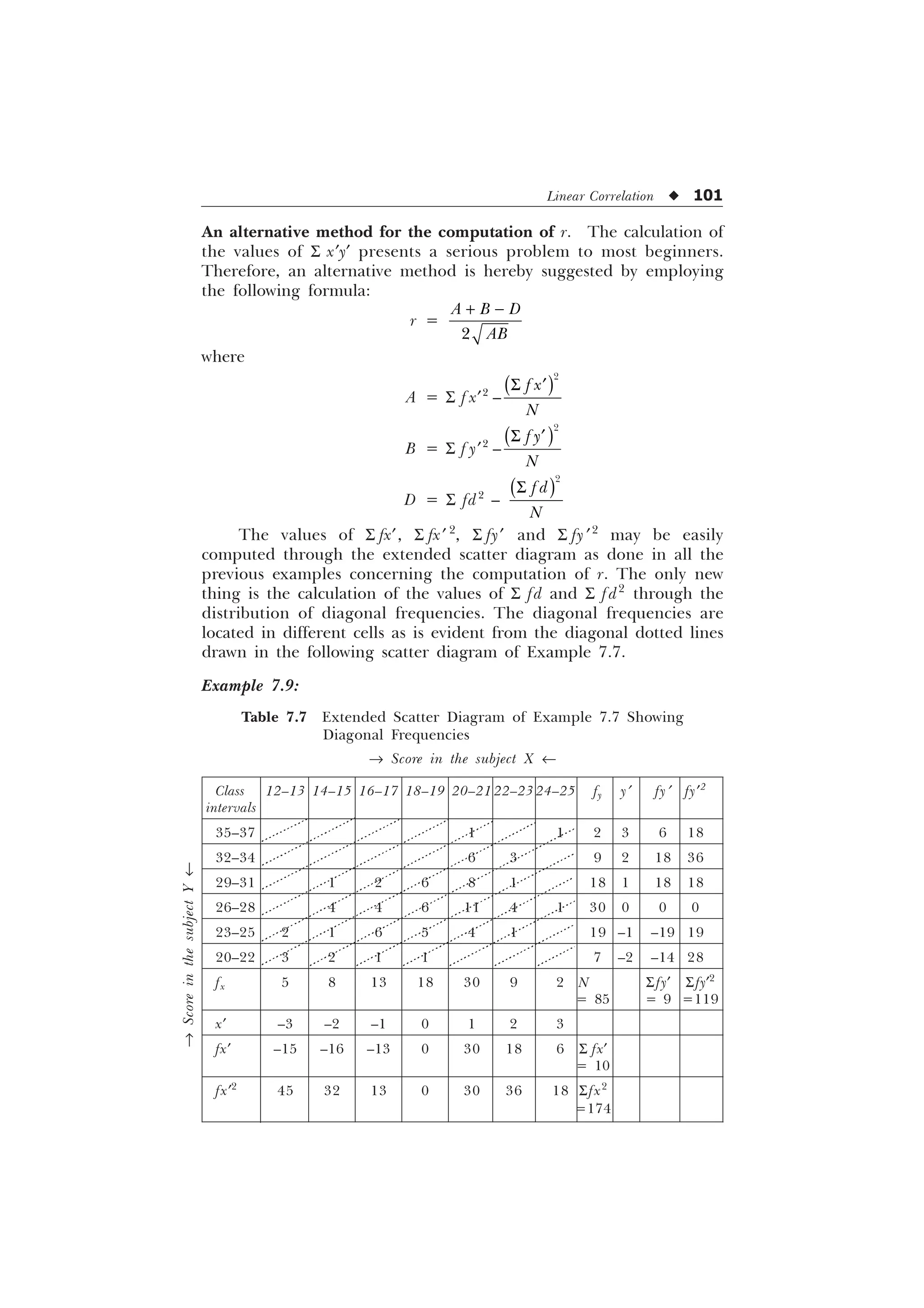
![Linear Correlation u 97
Solution: For solving the above given problem we will first work
for the extension of correlation table of the Example 7.7 and then
calculate the needed values of S x¢y¢, S fx¢, S fy¢, S fx¢2
, S fy¢2
etc. finally
for computing r. The extended table with the needed computation
work has been shown in Table 7.5.
Computation of r
r =
1 [ I [ I
1 I [ I [ 1 I I
6 6 ¹ 6
„ „ „ „
Ë Û Ë Û
6 6 6 6
„ „ „ „
Í Ý Í Ý
=
– –
– – – –
=
=
–
=
=
= 0.54 (approx.)
[Ans. Pearson’s correlation coefficient = 0.54.]](https://image.slidesharecdn.com/stats-s-241206101830-e3d4cc67/75/Stats-S-K-Mangal-statistics-textook-in-pdf-109-2048.jpg)
![Linear Correlation u 99
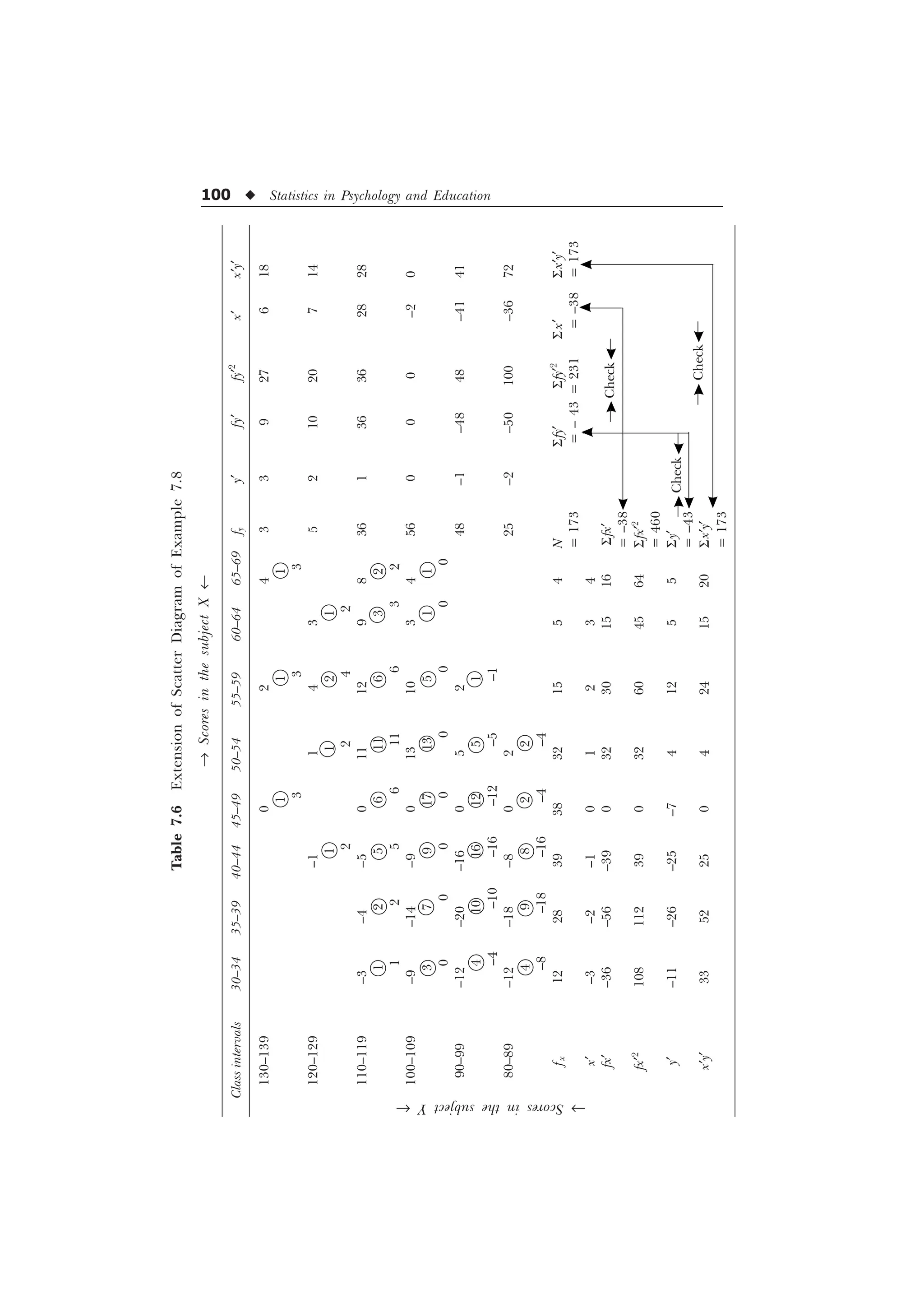
Example 7.8:
® Scores in the subject X ¬
Class 30–34 35–39 40–44 45–49 50–54 55–59 60–64 65–69 Total
intervals
130–139 1 1 1 3
120–129 1 1 2 1 5
110–119 1 2 5 6 11 6 3 2 36
100–109 3 7 9 17 13 5 1 1 56
90–99 4 10 16 12 5 1 48
80–89 4 9 8 2 2 25
Total 12 28 39 38 32 15 5 4 173
Solution: We will have extension of correlation table given in
Example 7.8 along with the computation of the needed values S x¢y¢,
S fx¢, S fy¢, S fx¢2
, S fy¢2
, as provided in Table 7.6.
Computation of r
r =
6 6 6
„ „ „ „
Ë Û Ë Û
6 6 6 6
„ „ „ „
Í Ý Í Ý
1 [ I [ I
1 I [ I [ 1 I I
=
– –
Ë Û Ë Û
– – – –
Í Ý Í Ý
=
=
–
=
=
= 0.518
= 0.52 (approx.)
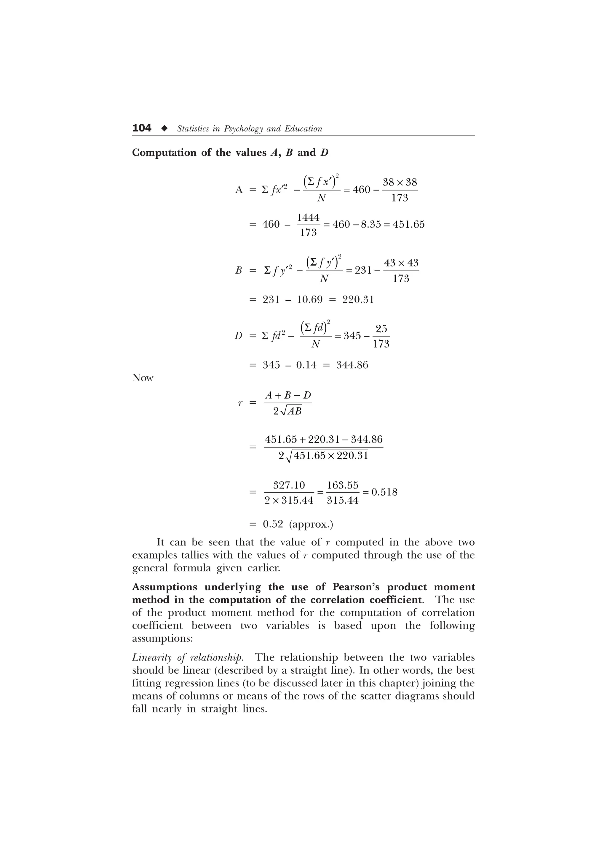
[Ans. Pearson’s correlation coefficient = 0.52.]
®
Scores
in
the
subject
Y
¬](https://image.slidesharecdn.com/stats-s-241206101830-e3d4cc67/75/Stats-S-K-Mangal-statistics-textook-in-pdf-111-2048.jpg)
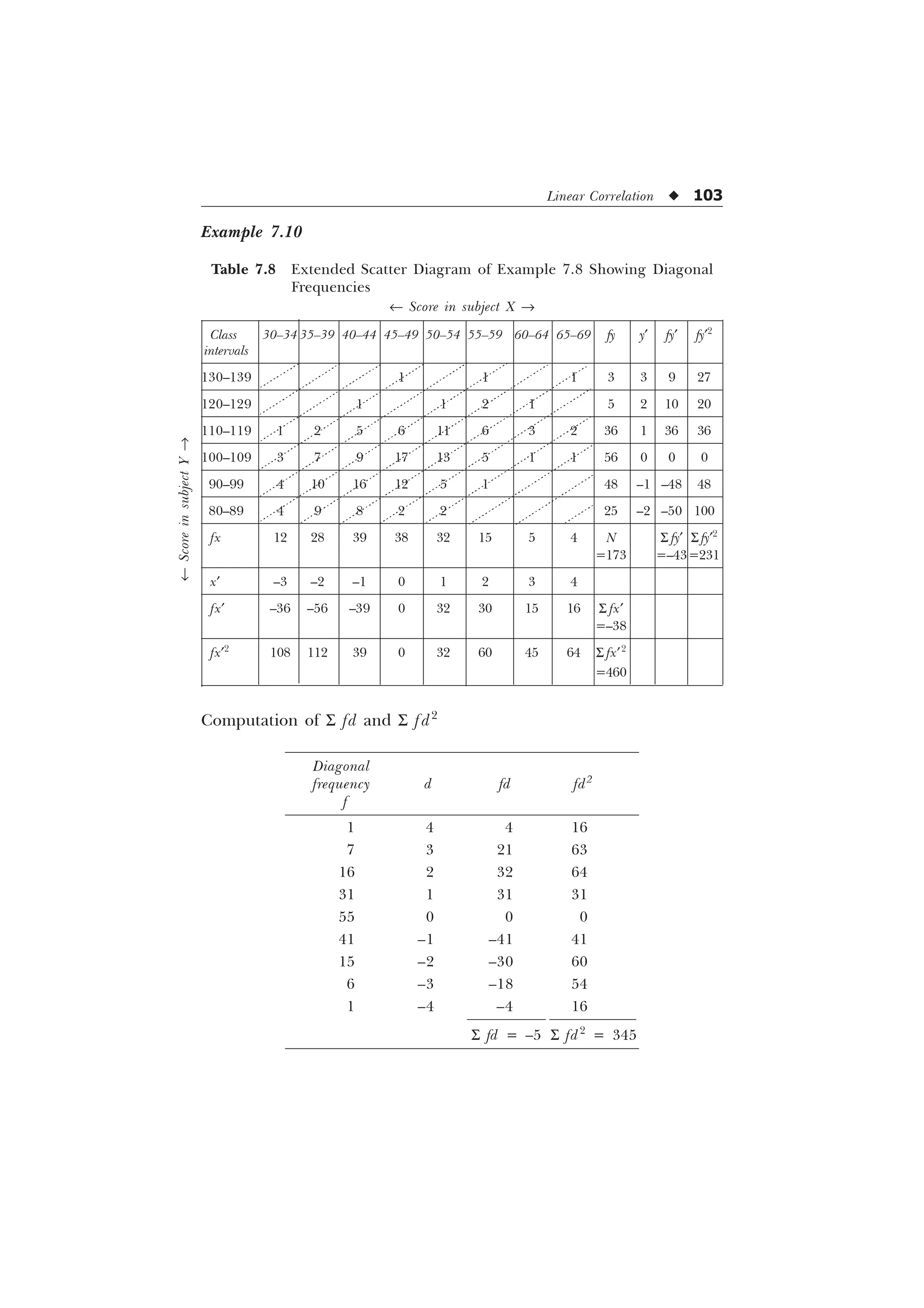
![102 u Statistics in Psychology and Education
The frequencies in the respective diagonal cells may be easily
located along the dotted lines of the above scatter diagram and the
process of the computation of the values of S fd and S fd2
may be
carried out as follows:
Diagonal
frequency d fd fd2
f
1 3 3 9
9 2 18 36
20 1 20 20
16 0 0 0
18 –1 –18 18
9 –2 –18 36
2 –3 –6 18
N = 85 S fd = –1 S fd2
= 137
The values of A, B and D can now be calculated as follows
A =
6 „
6
„
I [
I [
1
= 174 – 1.18 = 172.82
B =
6 „
6
„
I
I
1
= 119 – 0.95 = 118.05
D =
6
6
IG
IG
1
= 137 –
= 137 – 0.01
= 136.99
r =
$ % '
$%
=
–
=
–
=
= 0.539 = 0.54 (approx.)
[Ans. Product moment correlation coefficient = 0.54.]](https://image.slidesharecdn.com/stats-s-241206101830-e3d4cc67/75/Stats-S-K-Mangal-statistics-textook-in-pdf-114-2048.jpg)
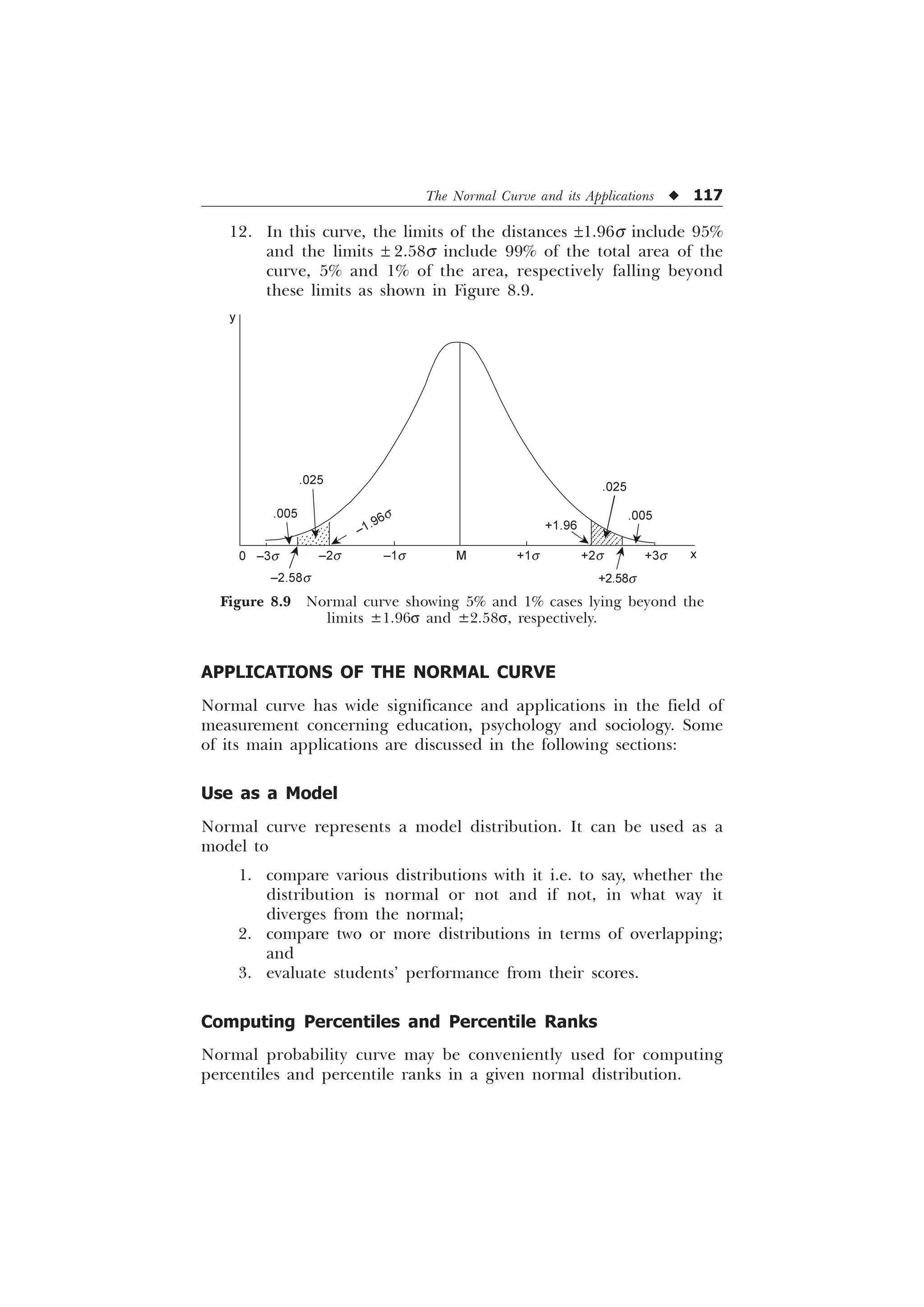
![118 u Statistics in Psychology and Education
Understanding and Applying the Concept of Standard
Errors of Measurement
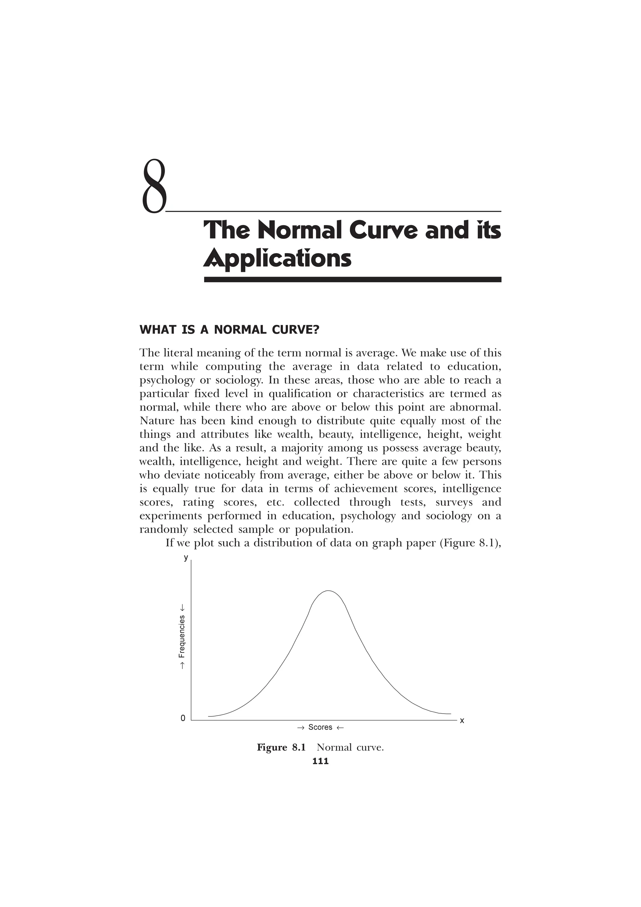
The normal curve as we have pointed out earlier, is also known as
the normal curve of error or simply the curve of error on the grounds
that it helps in understanding the concept of standard errors of
measurement. For example, if we compute mean for the distributions
of various samples taken from a single population, then, these means
will be found to be distributed normally around the mean of the entire
population. The sigma distance of a particular sample mean may help
us determine the standard error of measurement for the mean of that
sample.
Ability Grouping
A group of individuals may be conveniently grouped into certain
categories as A, B, C, D, E (Very good, good, average, poor, very poor)
in terms of some trait (assumed to be normally distributed), with the
help of a normal curve.
Transforming and Combining Qualitative Data
Under the assumption of normality of the distributed variable, the sets
of qualitative data such as ratings, letter grades and categorical ranks
on a scale may be conveniently transformed and combined to provide
an average rating for each individual.
Converting Raw Scores into Comparable Standard
Normalized Scores
Sometimes, we have records of an individual’s performance on two or
more different kinds of assessment tests and we wish to compare his
score on one test with the score on the other. Unless the scales of these
two tests are the same, we cannot make a direct comparison. With the
help of a normal curve, we can convert the raw scores belonging to
different tests into standard normalized scores like sigma (or z scores)
and T-scores. For converting a given raw score into a z score, we
subtract the mean of the scores of the distribution from the respective
raw scores and divide it by the standard deviation of the distribution
LH
; 0
]
T
È Ø
É Ù
Ê Ú . In this way, a standard z score clearly indicates how
many standard deviation units a raw score is above or below the mean
and thus provides a standard scale for the purpose of valuable](https://image.slidesharecdn.com/stats-s-241206101830-e3d4cc67/75/Stats-S-K-Mangal-statistics-textook-in-pdf-130-2048.jpg)
![120 u Statistics in Psychology and Education
]
Example 8.2: Given M = 48, s = 8, for a distribution, convert a z
score (s score) of the value 0.625 into a raw score.
Solution
; 0
]
T
Putting known values in the given formula, we get
0.625 =
;
or
X = 0.625 ´ 8 + 48 = 5.0 + 48 = 53
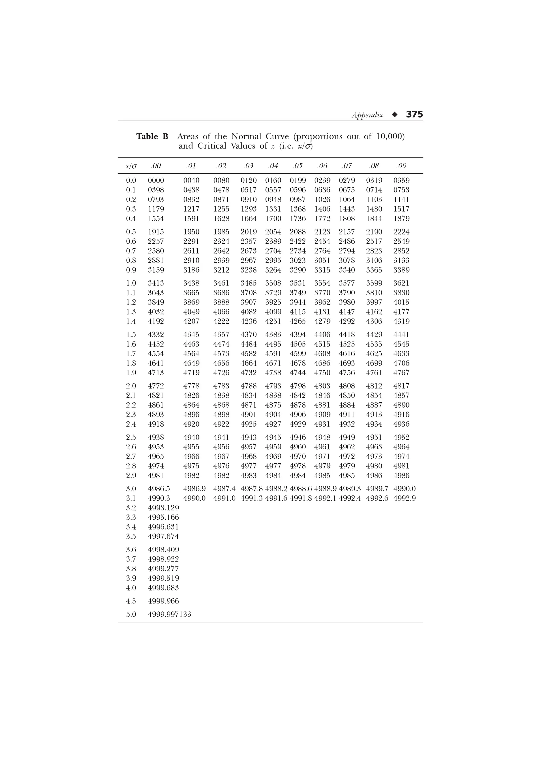
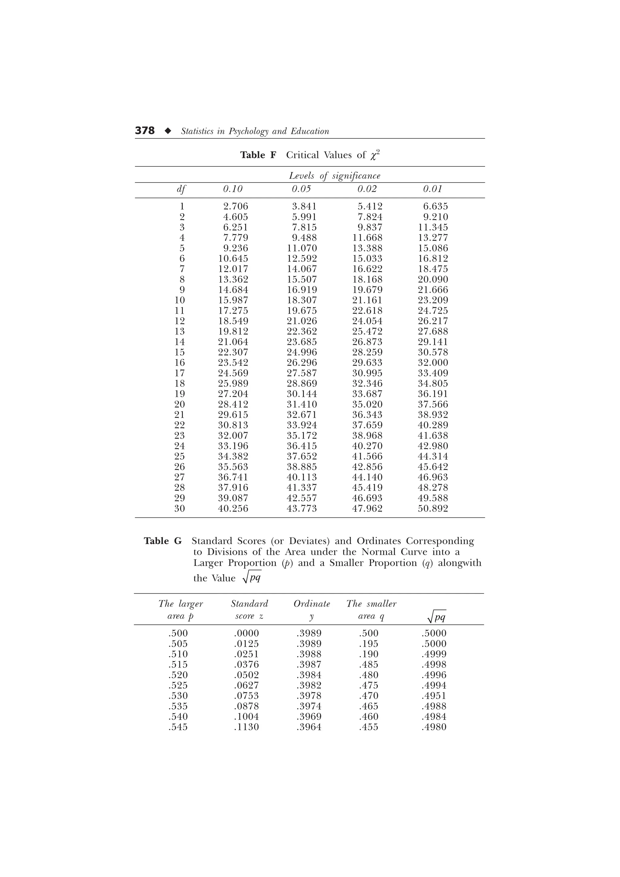
Making Use of the Table of Normal Curve
Table B of the normal curve (given in the Appendix) provides the
fractional parts of the total area (taken as 10,000) under the curve in
relation to the respective sigma distances from the mean. This table
may therefore be used to find the fractional part of the total area when
z scores or sigma scores are given and also to find the sigma or z scores,
when the fractional parts of the total area are given. Let us illustrate
it with the help of examples.
Example 8.3: From the table of the normal distribution, read the
areas from mean to 2.73s.
Solution. We have to look for the figure of the total area given
in the table corresponding to 2.73s score. For this we have to first
locate 2.7 sigma distance in the first column headed by
; 0
]
T
(s scores) and then move horizontally in the row against 2.7 until we
reach the place below the sigma distance .03 (lying in column 4). The
figure 4968 gives the fractional parts of the total area (taken as 10000)
corresponding to the 2.73s distance (lying on the right side) from the
mean of the curve. Consequently, 4968/10000 or 49.68 percent of the
cases may be said to lie between the mean and 2.73s.
Example 8.4: From the table of the normal distribution read the value
of sigma score from the mean for the corresponding fractional area
3729.](https://image.slidesharecdn.com/stats-s-241206101830-e3d4cc67/75/Stats-S-K-Mangal-statistics-textook-in-pdf-132-2048.jpg)
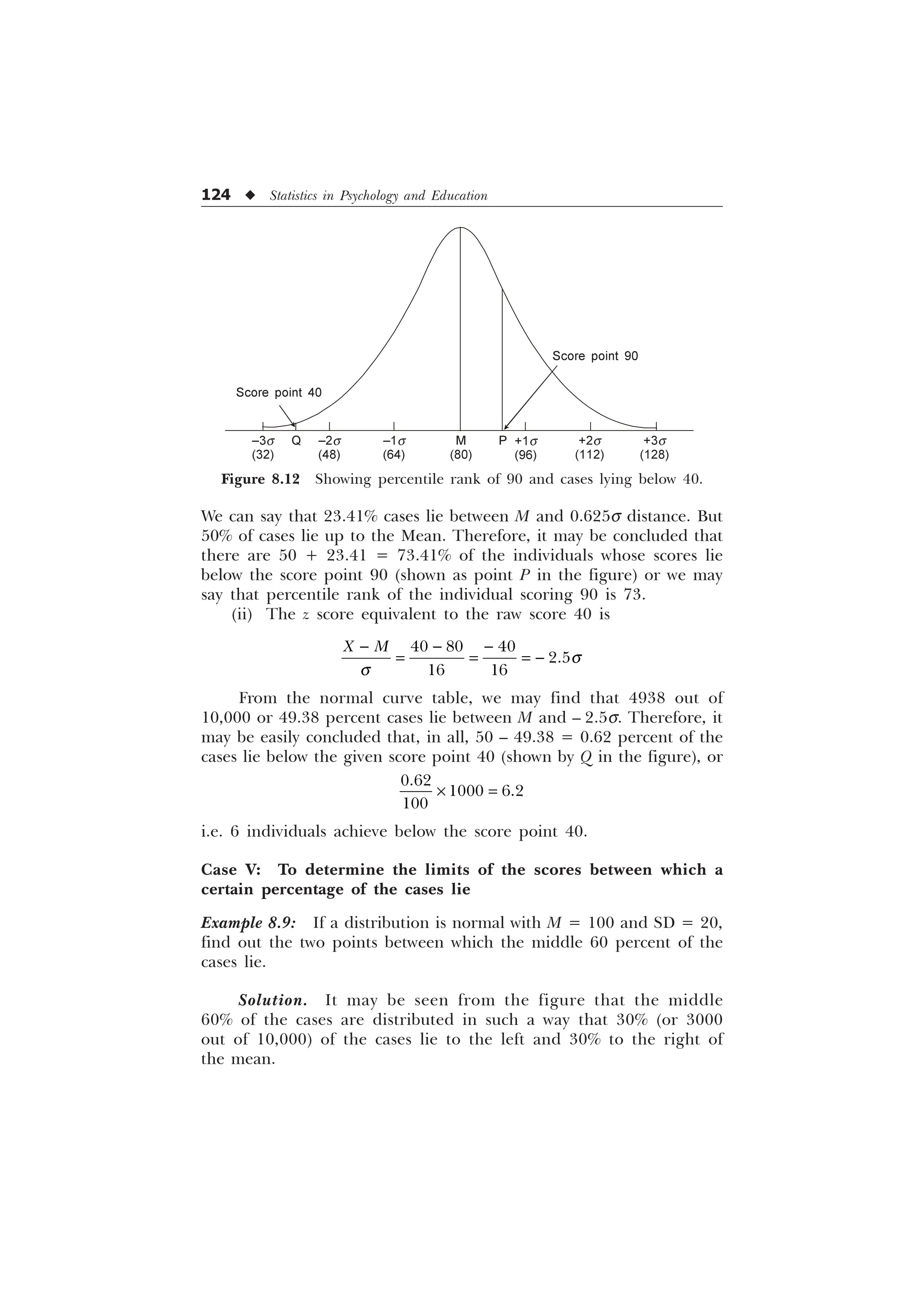
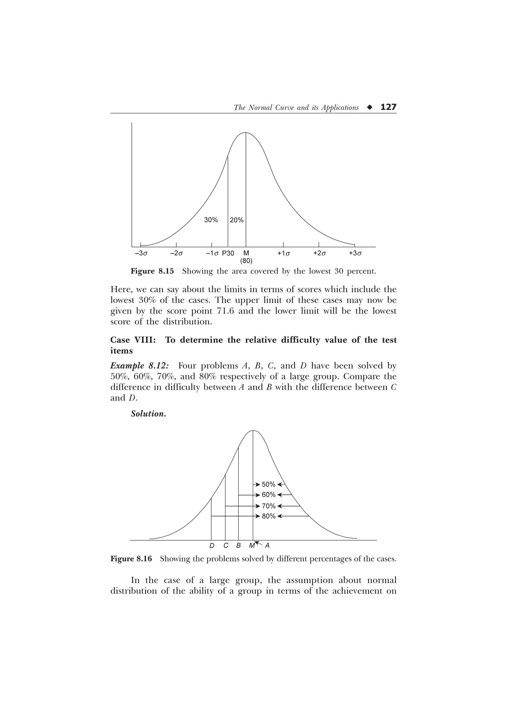
![The Normal Curve and its Applications u 125
From the normal curve (Table B in the Appendix), we have to
find out the corresponding s distance for the 3000 fractional parts of
the total area under the normal curve. There is a figure of 2995 for
area in the table (very close to 3000) for which we may read sigma
value as 0.84s. It means that 30% of the cases lie on the right side of
the curve between M and 0.84s and similarly 30% of the cases lie on
the left side of the figure between M and –0.84s. The middle 60% of
the cases, therefore, fall between the mean and standard score +0.84s.
We have to convert the standard z scores to raw scores with the help
of the formulae
z =
T T
; 0
; 0
]
or
0.48 =
DQG
;
;
or
X1 = 16.8 + 100 and X2 = 100 – 16.8
or
X1 = 116.8 and X2 = 83.2
After rounding the figures, we have the scores 117 and 83 that
include the middle 60 percent of the cases.
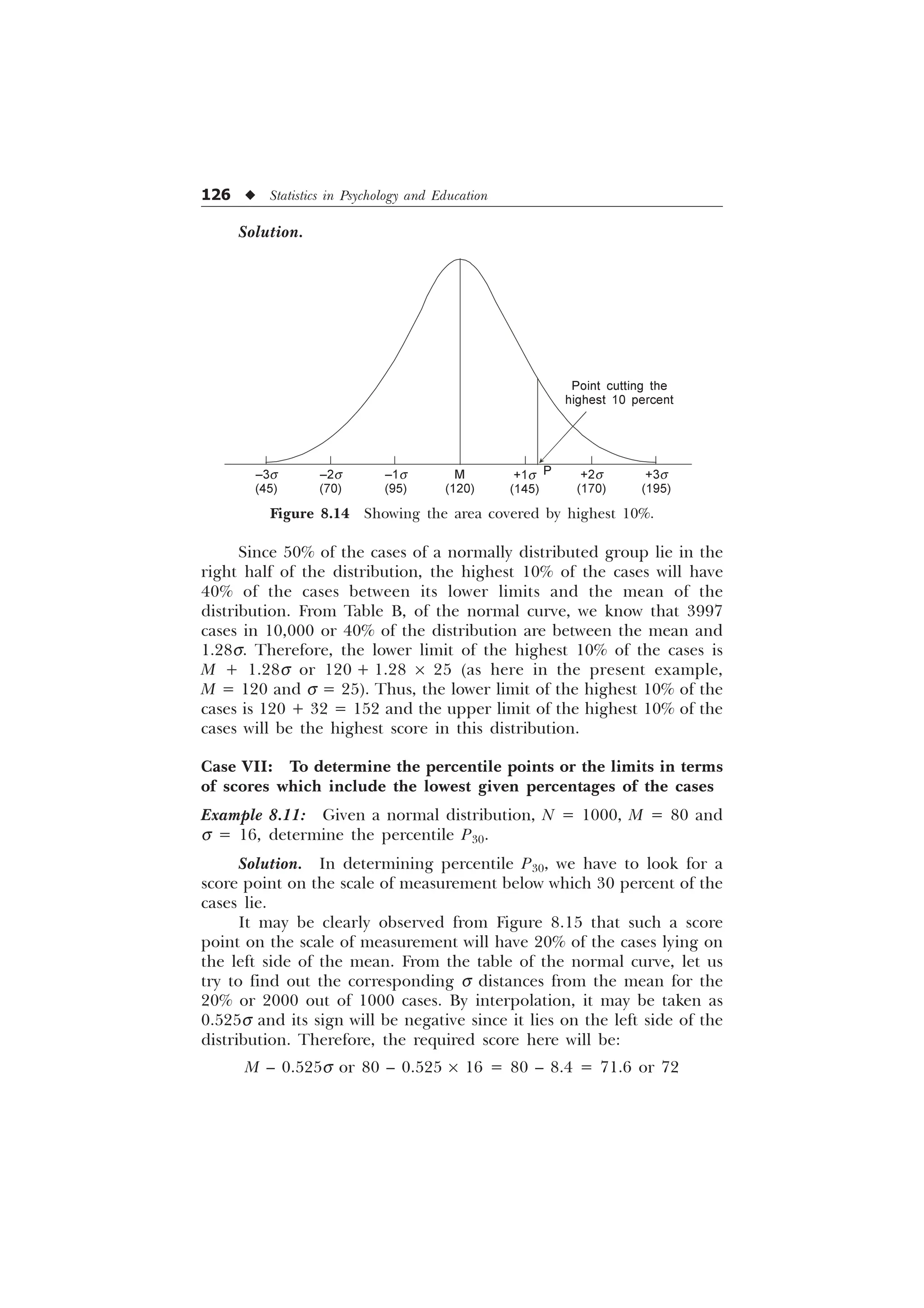
Case VI: To find out the limits in terms of scores which include
the highest given percentages of the cases
Example 8.10: Given a normal distribution with a mean of 120 and
SD of 25, what limits will include the highest 10% of the distribuution
(see Figure 8.14).
Figure 8.13 Showing the area covered by middle 60 percent.
+1s
(120)
+2s
(140)
+3s
(160)
M
(100)
–1s
(80)
–2s
(60)
–3s
(40)
30% 30%
Total
60%](https://image.slidesharecdn.com/stats-s-241206101830-e3d4cc67/75/Stats-S-K-Mangal-statistics-textook-in-pdf-137-2048.jpg)
![158 u Statistics in Psychology and Education
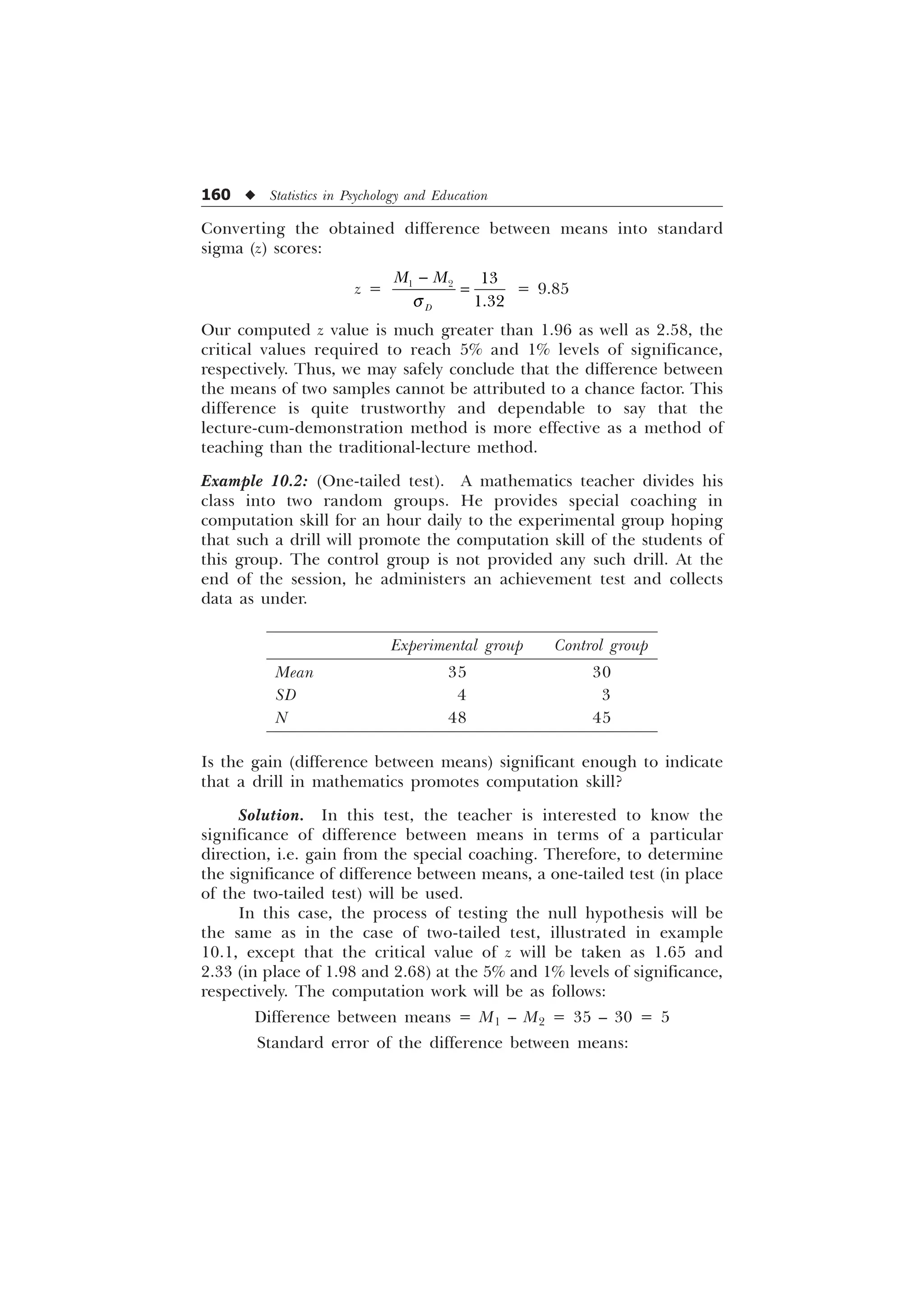
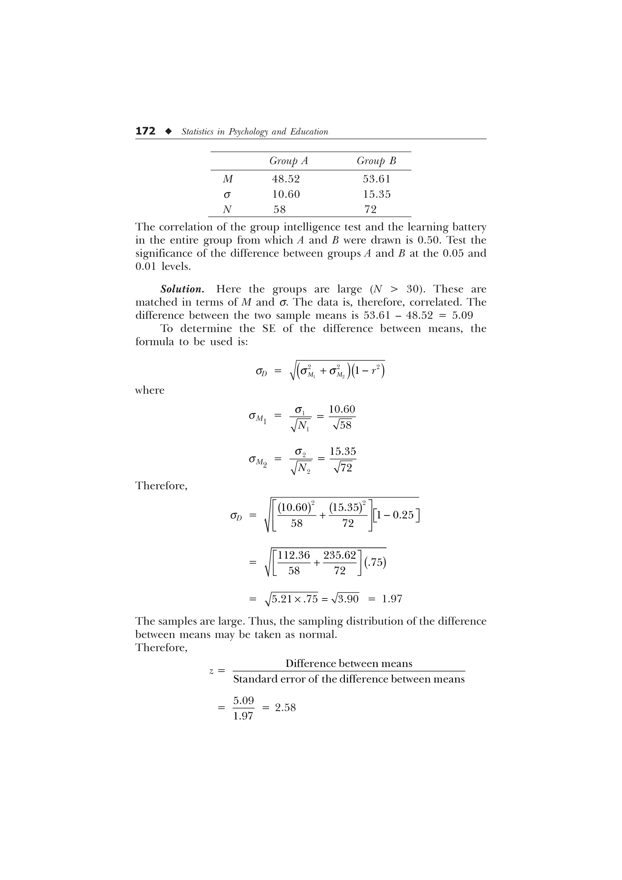
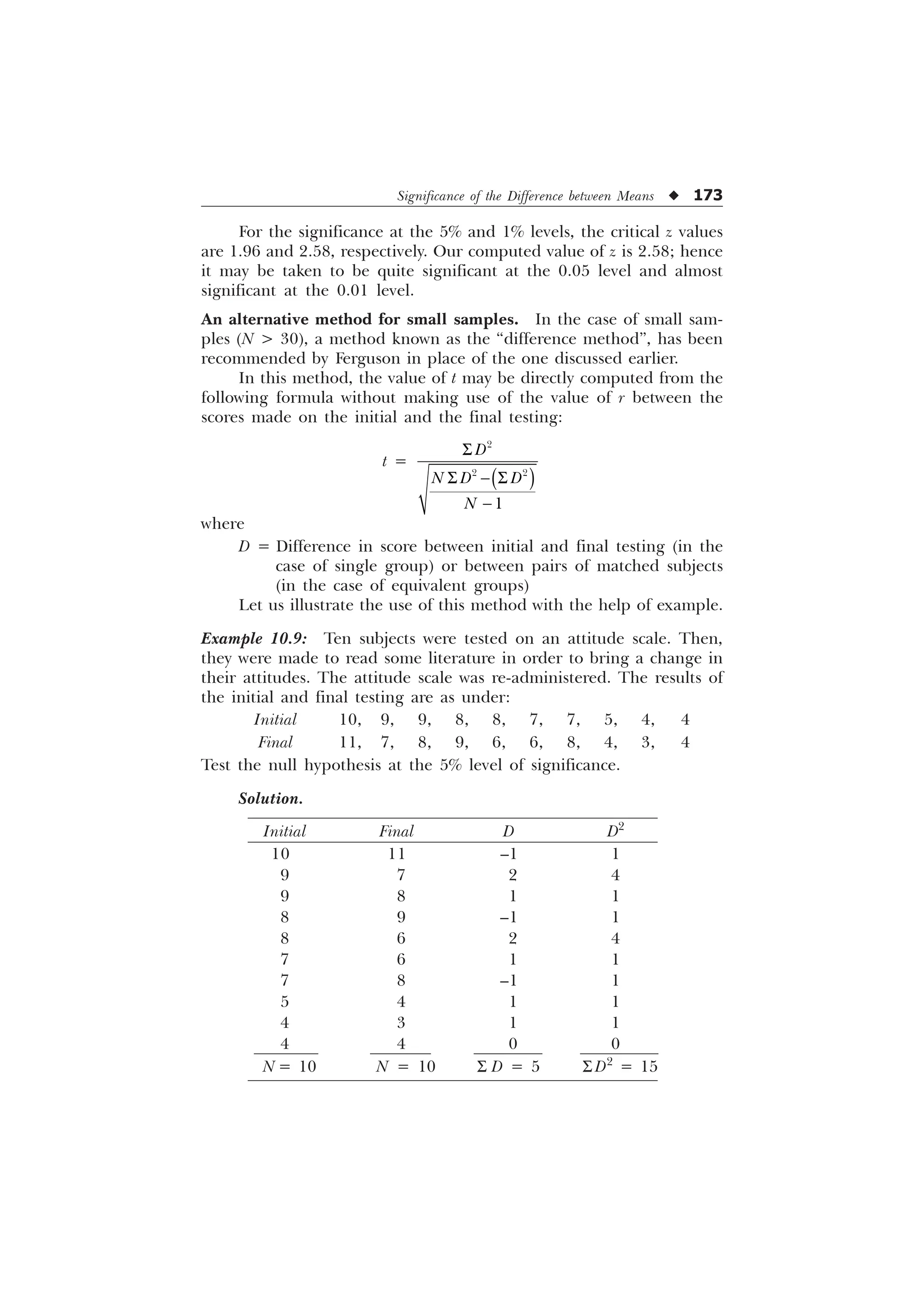
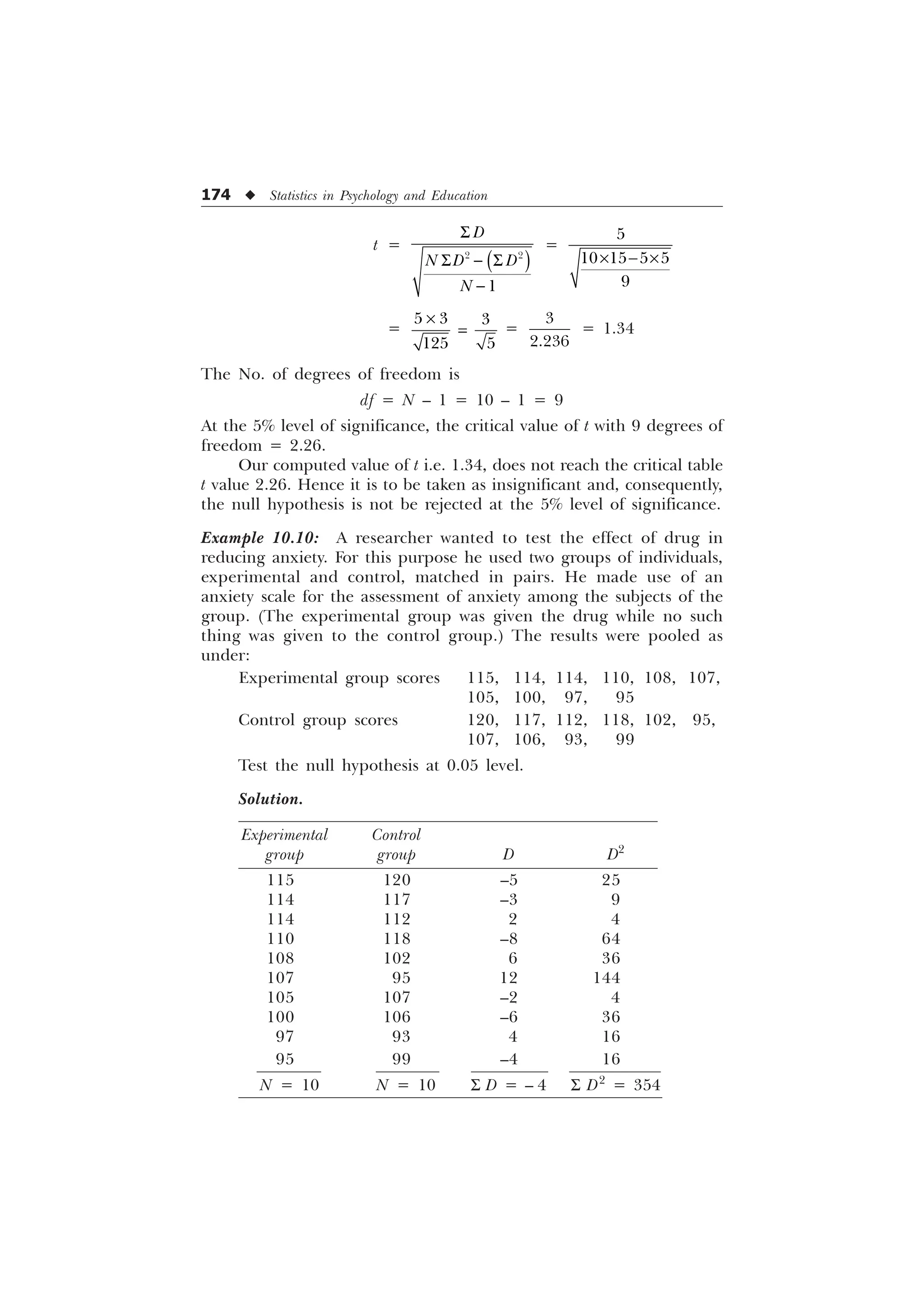
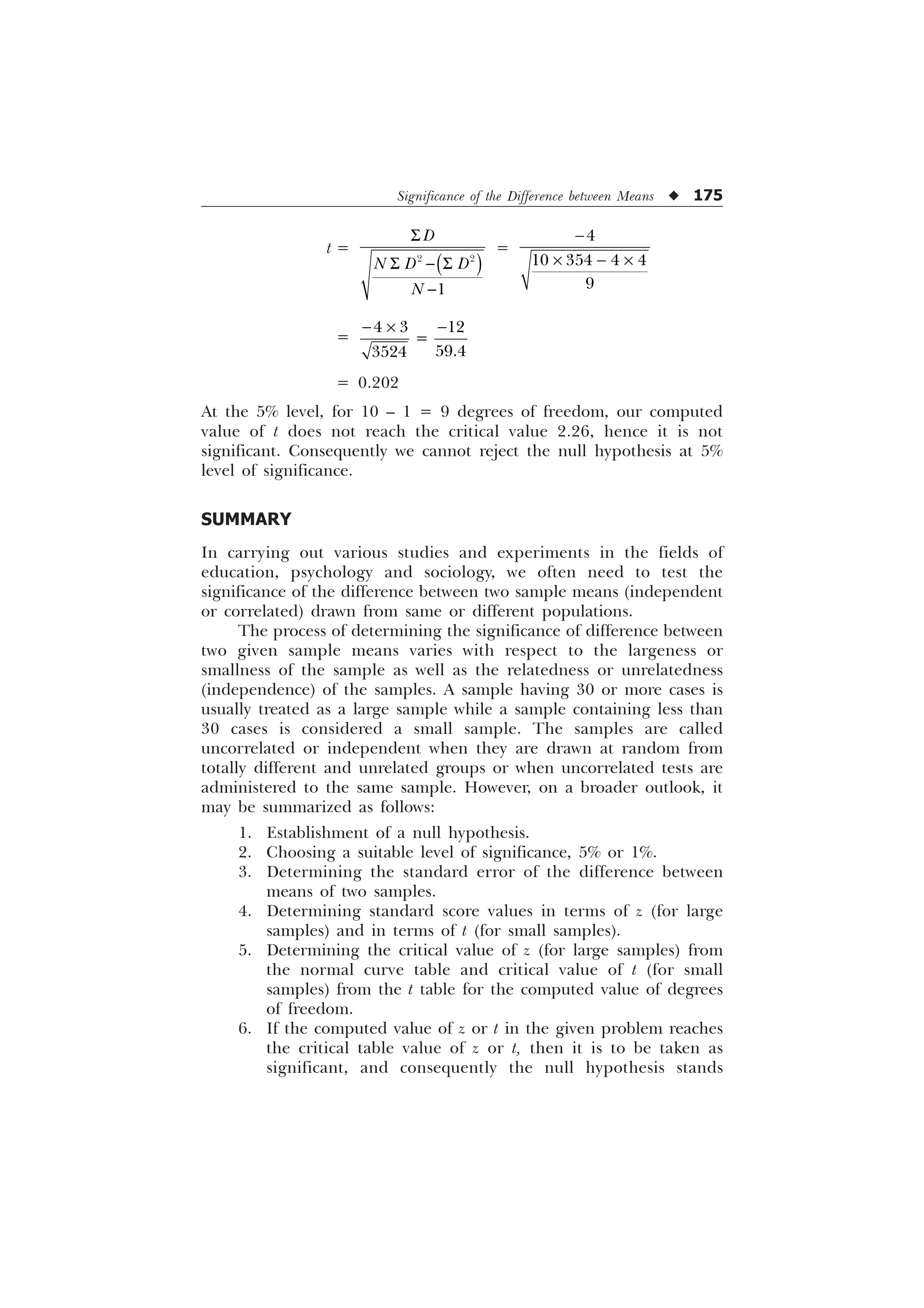
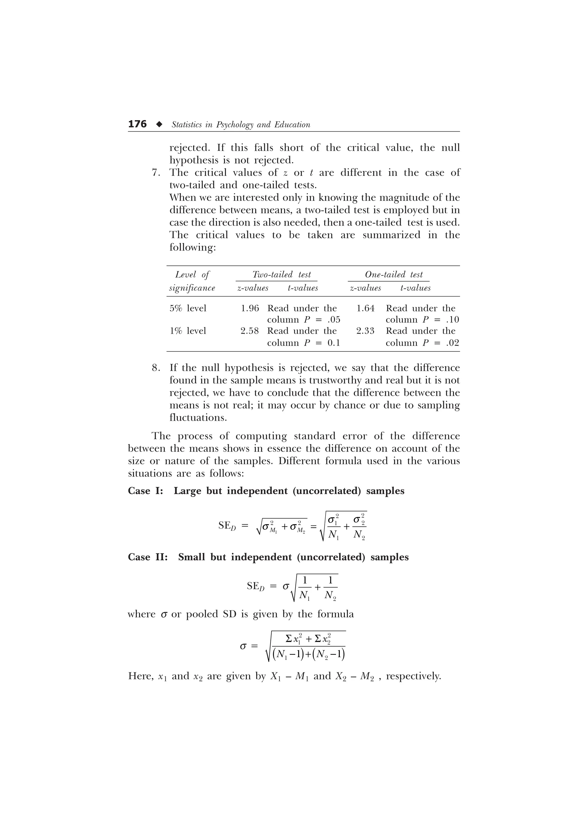
Step 1. To determine the SE of the difference between the means of two samples.
The formula for determining standard error of the difference between
means of two large but independent (non-correlated) samples is:
SED or sD =
0 0
T T
where
sM1
= SE of the means of the first sample
sM2
= SE of the means of the second sample
As we already know, sM1
and sM2
may be calculated by the formula
sM1
=
1
T
where s1 is the SD of the first sample and N1 is the size of the first
sample.
sM2
=
1
T
where s2 is the SD of the second sample and N2 is the size of the
second sample. In this way, the formula becomes
sD =
1 1
T
T
Step 2. To compute the z value for the difference in sample means. The
sampling distribution of difference between means in the case of large
samples is a normal distribution. This difference represented on the
base line of the normal curve may be converted into standard sigma
scores (z values) with the help of the following formula:
z =
T
'LIIHUHQFHEHWZHHQPHDQV
6WDQGDUGHUURURIGLIIHUHQFHEHWZHHQPHDQV
'
0 0
In this way, z represents the ratio of difference between the means to
the standard error of the difference between the means.
Step 3. Testing the null hypothesis at some pre-established level of significance.
At this stage, the null hypothesis, i.e. there exists no real difference
between the two sample means, is tested against its possible rejection at
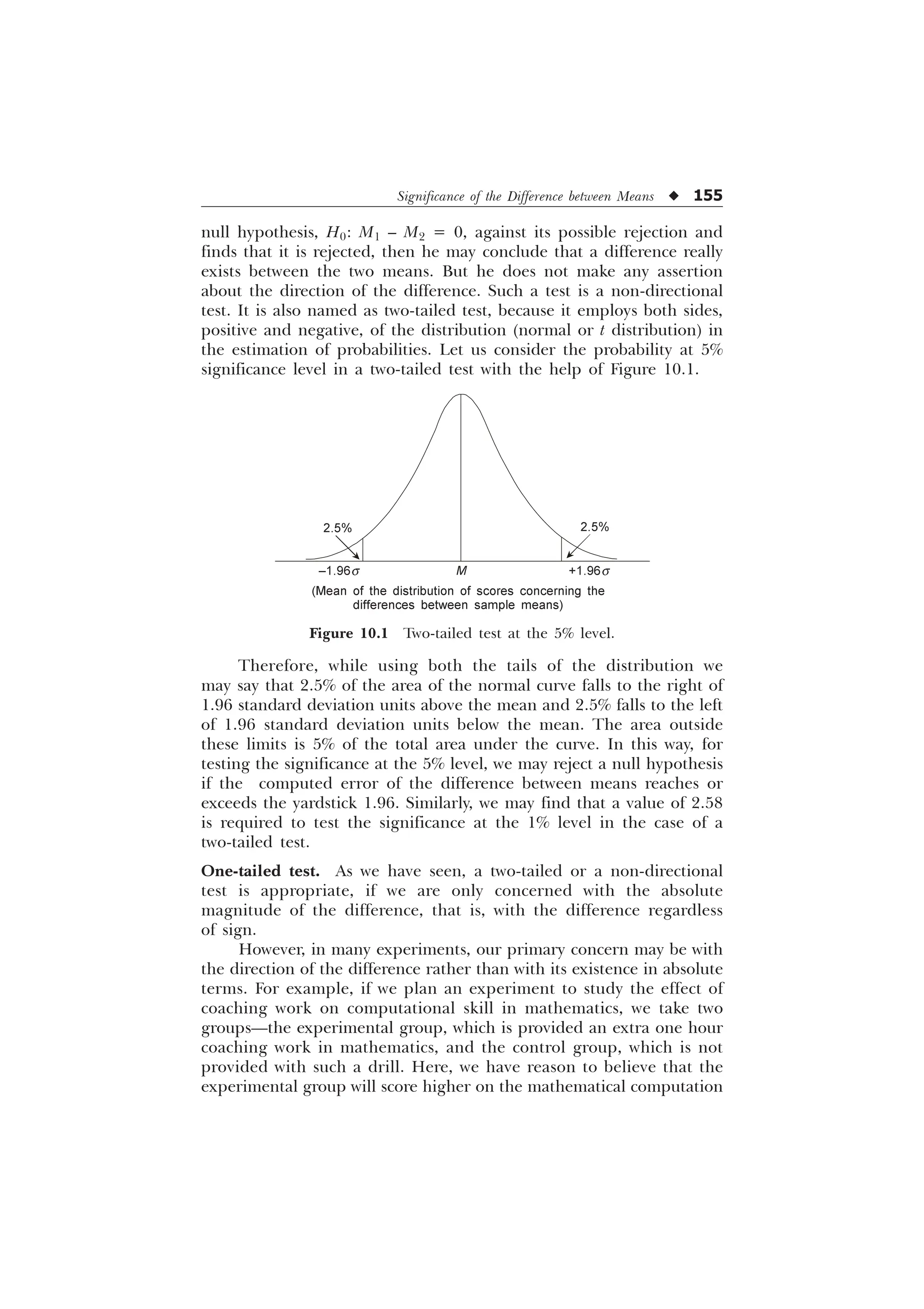
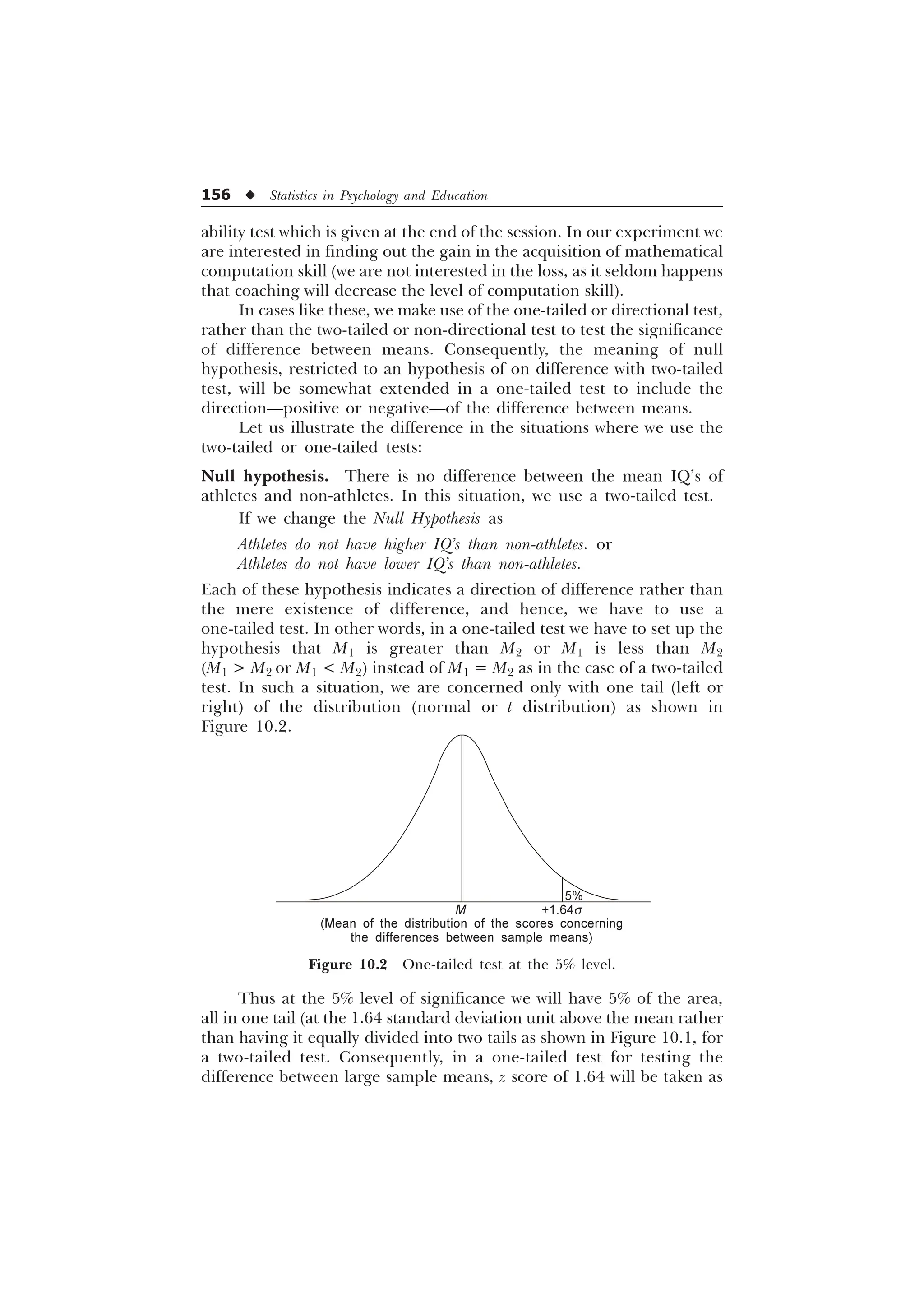
5% or 1% level of significance in the following manner.
1. If the computed z value [i.e. z = (M1 – M2)/sD] is equal to 19.6
or greater than 1.96 (equal to or greater than 1.65 in the case
of a one-tailed test), we declare it significant for the rejection
of the null hypothesis at 5% level of significance.](https://image.slidesharecdn.com/stats-s-241206101830-e3d4cc67/75/Stats-S-K-Mangal-statistics-textook-in-pdf-170-2048.jpg)
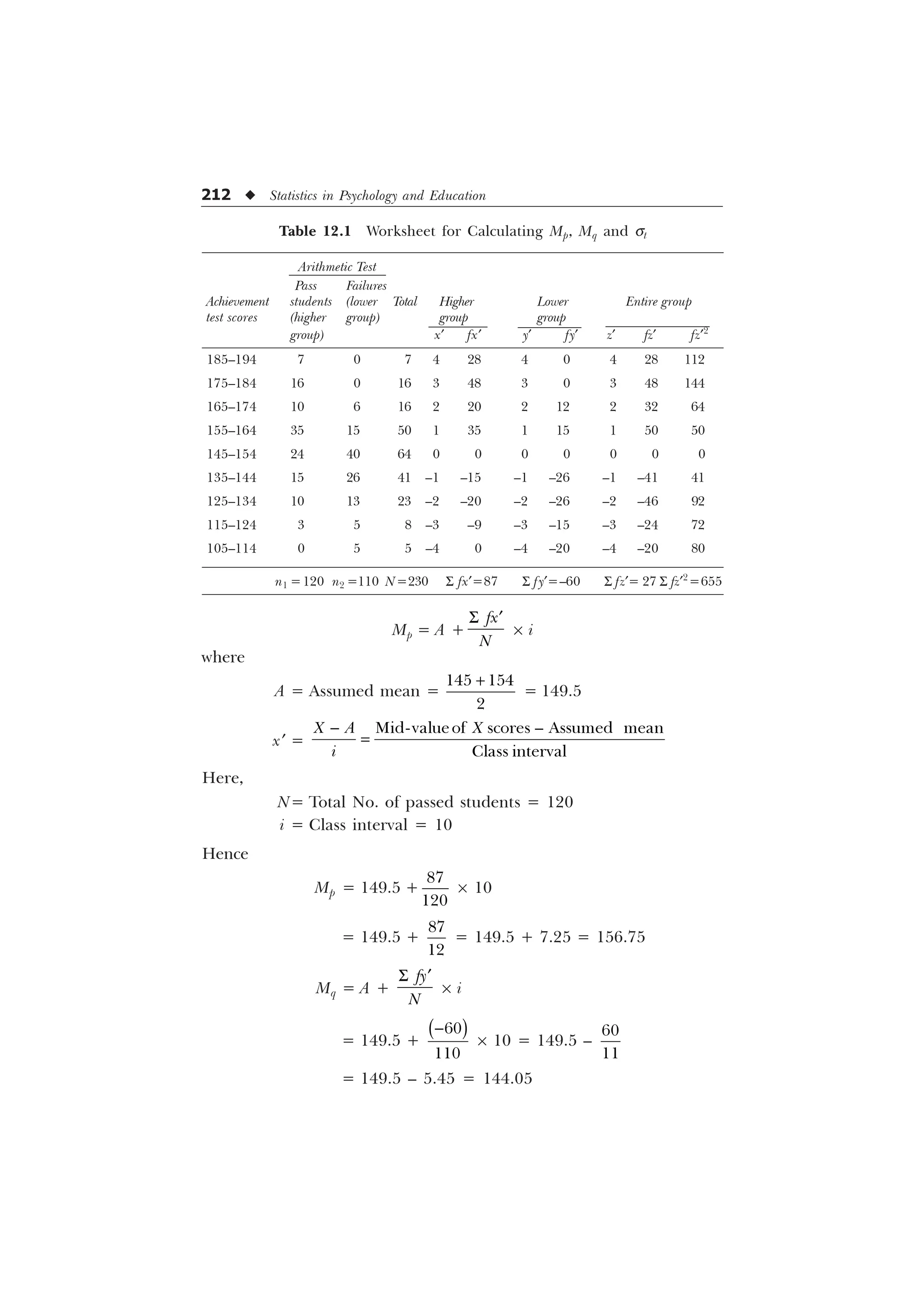
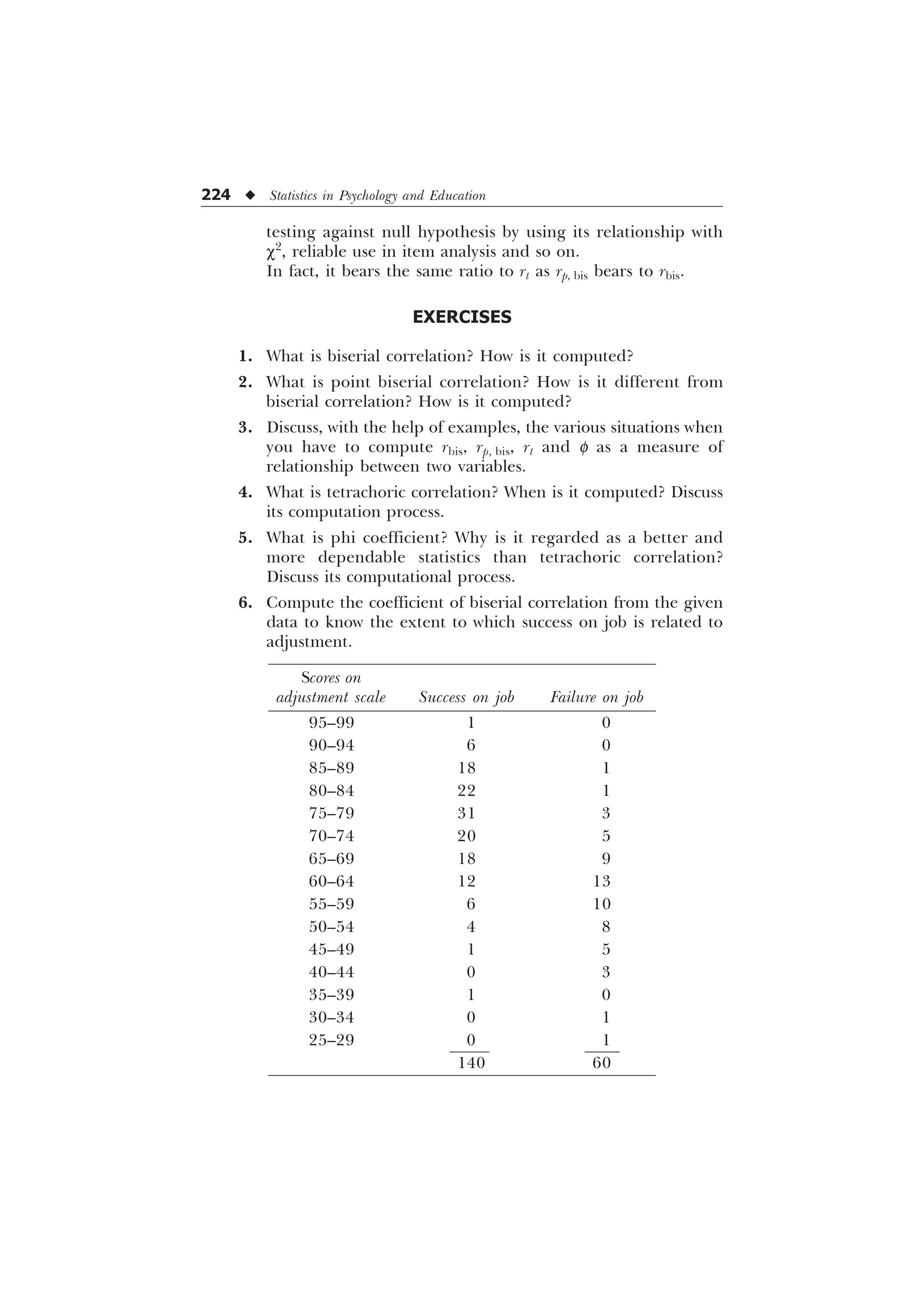
![Further Methods of Correlations u 213
Mp – Mq = 156.75 – 144.05 = 12.70
st = i
„ „
È Ø
É Ù
Ê Ú
I] I]
1 1
= 10
È Ø
É Ù
Ê Ú
= 10
–
–
=
– –
=
= 16.83
Step 5. Substitute the value of p, q, y, Mp, Mq and st in the following
formula:
rbis =
S T
W
0 0 ST
T
–
=
– –
–
=
– –
–
= 0.47
[Ans. Coefficient of biserial correlation, rbis = 0.47.]
Alternative Formula for rbis
The coefficient of biserial correlation, rbis, can also be computed with
the help of the following formula:
rbis =
S W
W
0 0 S
T
–
In this formula, we have to compute Mt (mean of the entire group) in
place of Mq.
Characteristics of Biserial Correlation
The biserial correlation coefficient, rbis, is computed when one variable](https://image.slidesharecdn.com/stats-s-241206101830-e3d4cc67/75/Stats-S-K-Mangal-statistics-textook-in-pdf-225-2048.jpg)
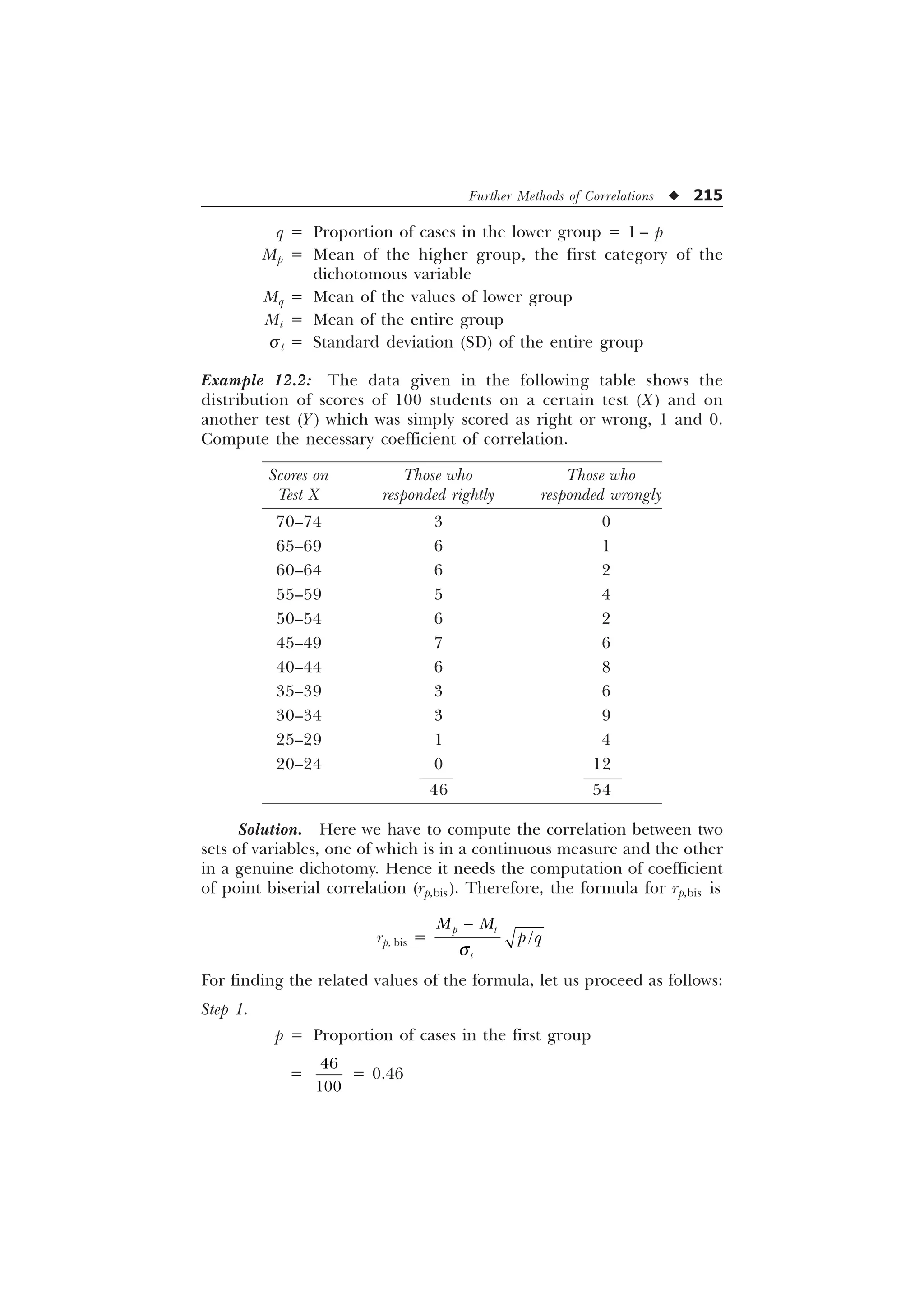
![216 u Statistics in Psychology and Education
Step 2. q = 1 – p = 1 – 0.46 = 0.54
Step 3. Calculation of Mp, Mt and st
The computation process is illustrated in Table 12.2
Table 12.2 Worksheet for Computation of Mp and st
Those who Those who
Scores responded responded Total x¢ fx¢ z¢ fz¢ fz¢2
on X rightly wrongly
70–74 3 0 3 5 15 5 15 75
65–69 6 1 7 4 24 4 28 112
60–64 6 2 8 3 18 3 24 72
55–59 5 4 9 2 10 2 18 36
50–54 6 2 8 1 6 1 8 8
45–49 7 6 13 0 0 0 0 0
40–44 6 8 14 –1 –6 –1 –14 14
35–39 3 6 9 –2 –6 –2 –18 36
30–34 3 9 12 –3 –9 –3 –36 108
25–29 1 4 5 –4 –4 –4 –20 80
20–24 0 12 12 –5 0 –5 –60 300
n1=46 n2 = 54 N=100 S fx¢=48 S fz¢=–55 S fz¢2
=841
Mp = A +
I[
Q
6 „
´ i = 47 +
´ 5 = 47 + 5.2 = 52.2
(Here, A = Assumed mean =
= 47, i = 5 and n1 = 46)
Mt = A +
I]
1
6 „
´ i= 47 +
´ 5 = 47 – 2.75 = 44.2
st = i
I] I]
1 1
6 6
„ „
È Ø
É Ù
Ê Ú
= 5
È Ø
É Ù
Ê Ú
= 5
–
–
=
=
=
= 14.236
rp,bis =
S W
W
0 0
S T
T
=
=
= = 0.52
[Ans. Point biserial correlation coefficient rp,bis = 0.52.]](https://image.slidesharecdn.com/stats-s-241206101830-e3d4cc67/75/Stats-S-K-Mangal-statistics-textook-in-pdf-228-2048.jpg)
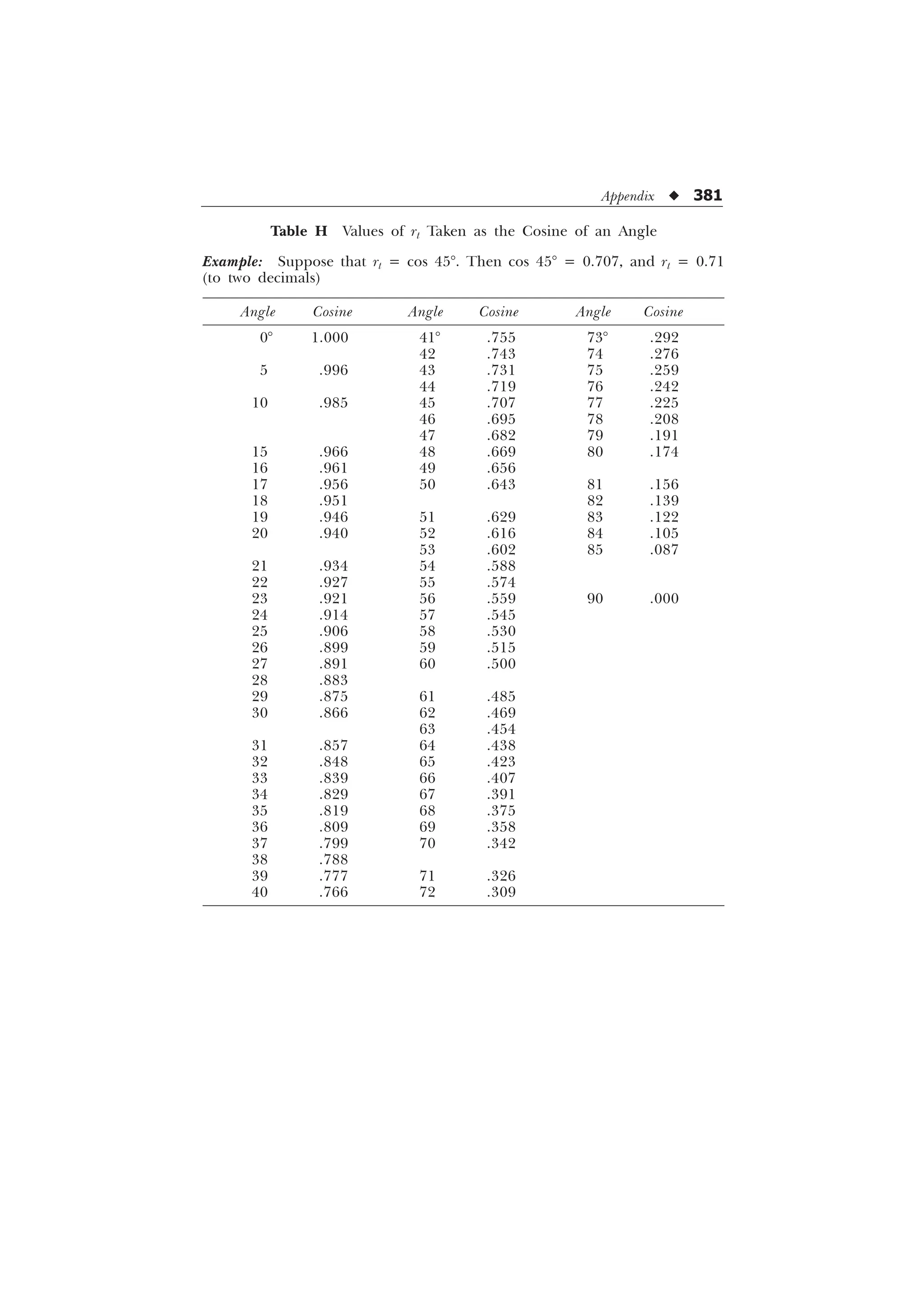
![220 u Statistics in Psychology and Education
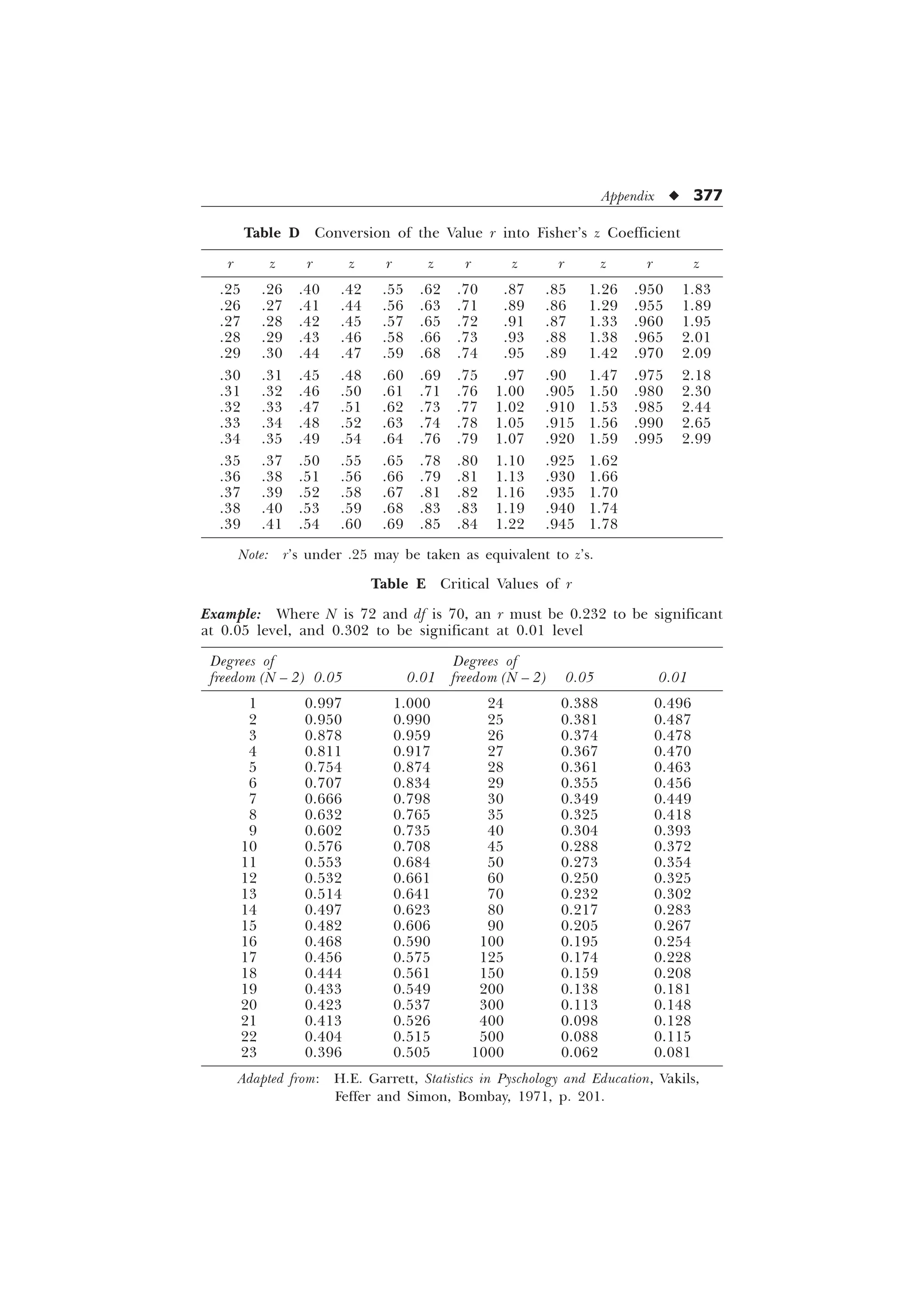
Step 3. Convert cos 82° into rt. (It can be done directly with the help
of Table H given in the Appendix.) Then,
rt = 0.139
[Ans. Tetrachoric correlation = 0.139.]
Limitations of the general formula rt = cos
%
$' %
È Ø
’ –
É Ù
Ê Ú
= cos
$' %
’
The foregoing formula shows good results in computation of rt
only when (i) N is large and (ii) the splits into dichotomized variables
are not far removed from the median.
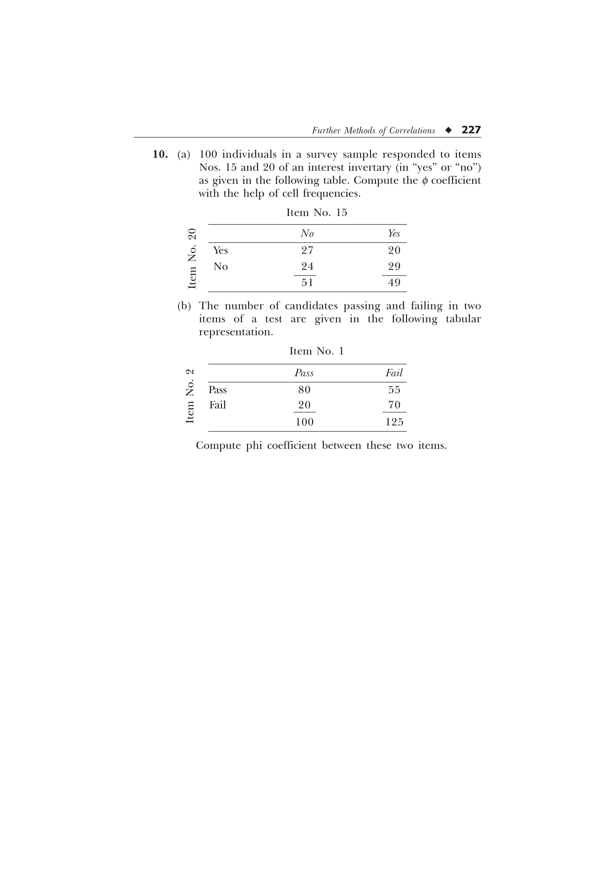
THE PHI (f) COEFFICIENT
In studies where we have to compute correlation between two such
variables which are genuinely dichotomous, it is the f coefficient that is
computed. Generally, its computation may involve the following
situations:
1. When the classification of the variables into two categories is
entirely and truly discrete, we are not allowed to have more
than two categories, i.e. living vs. dead, employed vs. not
employed, blue vs. brown eyes and so on.
2. When we have test items which are scored as Pass-Fail,
True-False, or opinion and attitude responses, which are
available in the form of yes-no, like-dislike, agree-disagree
etc., no other intermediate type of responses is allowed.
3. With such dichotomized variables which may be continuous
and may even be normally distributed, but are treated in
practical operations as if they were genuine dichotomies, e.g.
test items that are scored as either right or wrong, 1 and 0
and the like.
Computation of Phi (f) Coefficient
FORMULA. The formula for computation of f coefficient is
f =
%
$' %
$ ' % ' $](https://image.slidesharecdn.com/stats-s-241206101830-e3d4cc67/75/Stats-S-K-Mangal-statistics-textook-in-pdf-232-2048.jpg)
![Further Methods of Correlations u 221
where A, B, C, D represent the frequencies in the cells of the following
2 ´ 2 table:
X-variable
Yes No Total
Yes A B A + B
No C D C + D
Total A + C B + D A + B + C + D
Let us illustrate the use of forgoing formula with the help of an
example.
Example 12.4: There were two items X and Y in a test which were
responded by a sample of 200, given in the 2 ´ 2 table. Compute the
phi coefficient of correlation between these two items.
Solution.
Item X
Yes No Total
Yes 55 45 100
(A) (B) (A + B)
No 35 65 100
(C) (D) (C + D)
Total 90 110 200
(A + C) (B + D) (A + B + C + D)
FORMULA.
f coefficient =
%
$' %
$ ' % ' $
Substituting the respective values in the formula, we obtain
f =
– –
– – –
=
f =
= .201
[Ans. f coefficient = 0.201.]
Y-variable
Item
Y](https://image.slidesharecdn.com/stats-s-241206101830-e3d4cc67/75/Stats-S-K-Mangal-statistics-textook-in-pdf-233-2048.jpg)
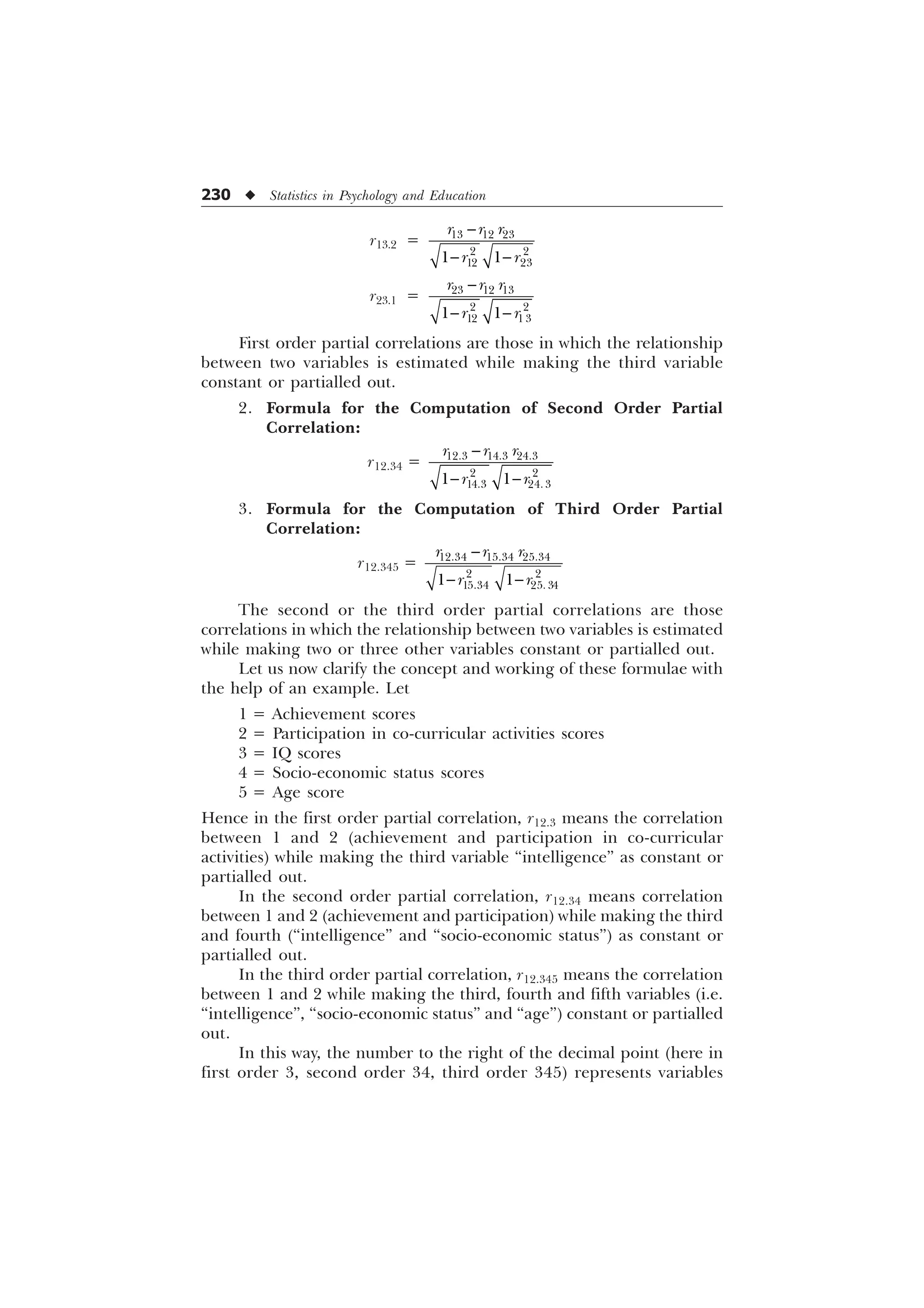
![Partial and Multiple Correlation u 231
whose influence is ruled out and the number to the left (here 12)
represents those two variables whose relationship needs to be estimated.
It is also clear from the given formulae that, for computation of
second order correlations, all the necessary first order correlations have
to be computed, and for the third order correlations, the second order
correlations must be known.
Let us now illustrate the process of computation of partial
correlation with the help of examples.
Example 13.1: From a certain number of schools in Delhi, a sample of
500 students studying in classes IX and X was taken. These students were
evaluated in terms of their academic achievement and participation in
co-curricular activities. Their IQ’s were also tested. The correlation
among these three variables was obtained and recorded as follows:
r12 = 0.18, r23 = 0.70, r13 = 0.60
Find out the independent correlation between the main (first two)
variables—academic achievement and participation—in co-curricular
activities.
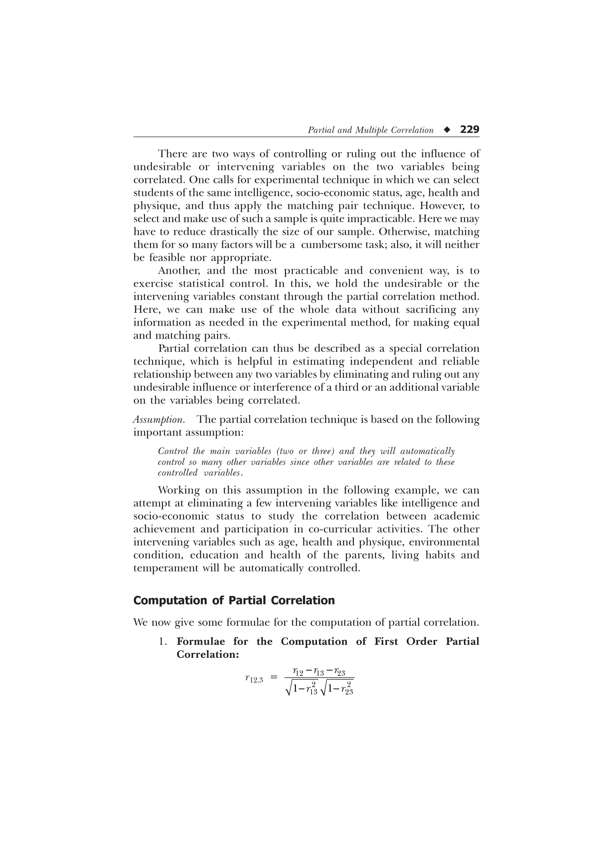
Solution. The independent and reliable correlation between
academic achievement and participation in co-curricular activities—the
main two variables—can be found by computing partial correlation
between these two variables, i.e. by computing r12.3 (keeping constant the
third variable)
r12.3 =
U U U
U U
Substituting the given value of correlation in the foregoing formula, we
obtain
r12.3 =
–
– –
=
=
–
=
= 0.67
[Ans. Partial correlation = 0.67.]](https://image.slidesharecdn.com/stats-s-241206101830-e3d4cc67/75/Stats-S-K-Mangal-statistics-textook-in-pdf-243-2048.jpg)
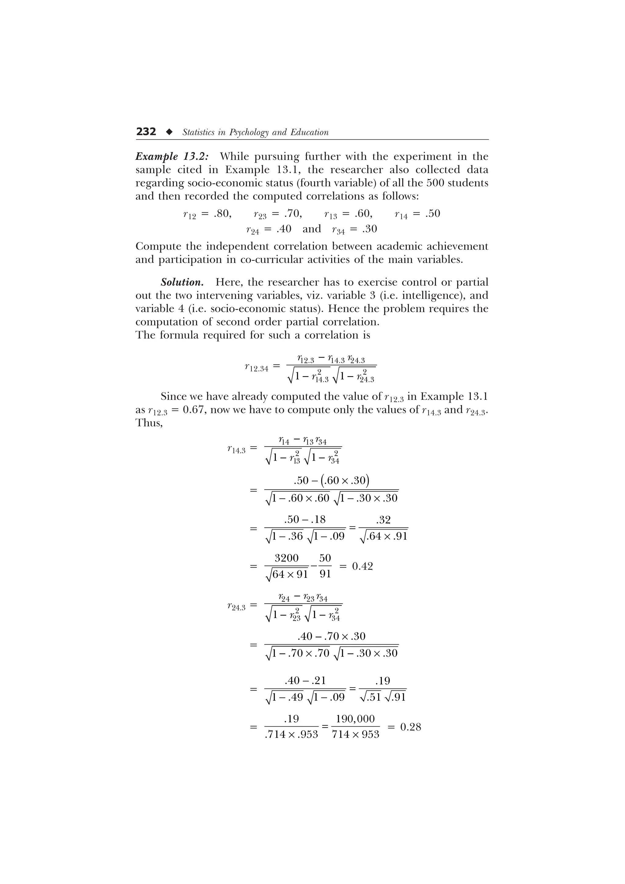
![Partial and Multiple Correlation u 233
r12.34 =
–
– –
=
=
–
=
= .64
[Ans. Partial correlation = 0.64.]
Application of Partial Correlation
Partial correlation can be used as a special statistical technique for
eliminating the effects of one or more variables on the two main
variables, for which we want to compute an independent and a reliable
measure of correlation. Besides its major advantage lies in the fact that
it enables us to set up a multiple regression equation (see Chapter 14)
of two or more variables, by means of which we can predict another
variable or criterion.
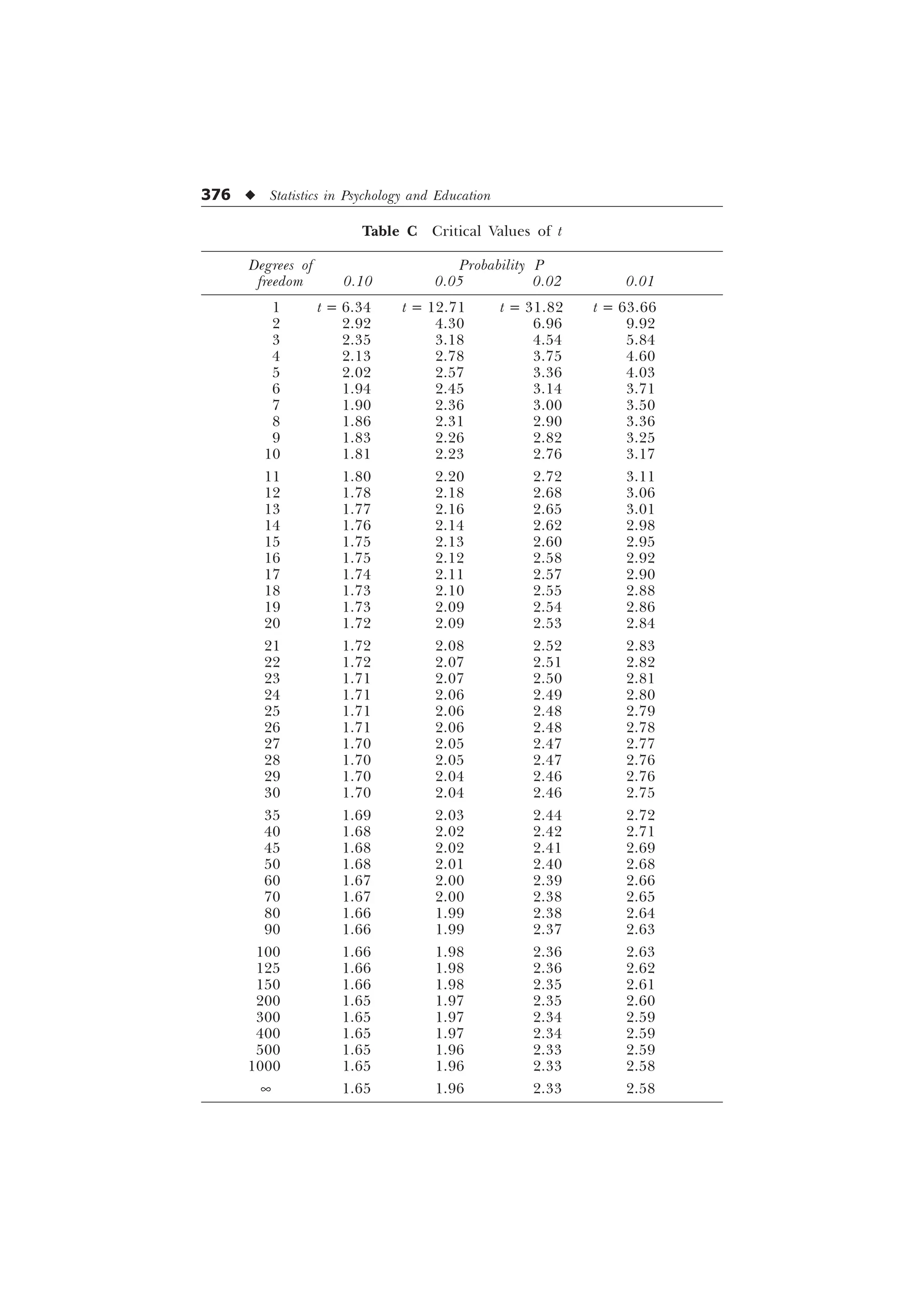
Significance of Partial Correlation Coefficient
The significance of the first and the second order partial correlation ‘r’
can be tested easily by using the ‘t’ distribution
t = r
1 .
U
where
K = Order of partial r
r = Value of partial correlation
N = Total frequencies in the sample study
Therefore,
Degree of freedom = N – 2 – K
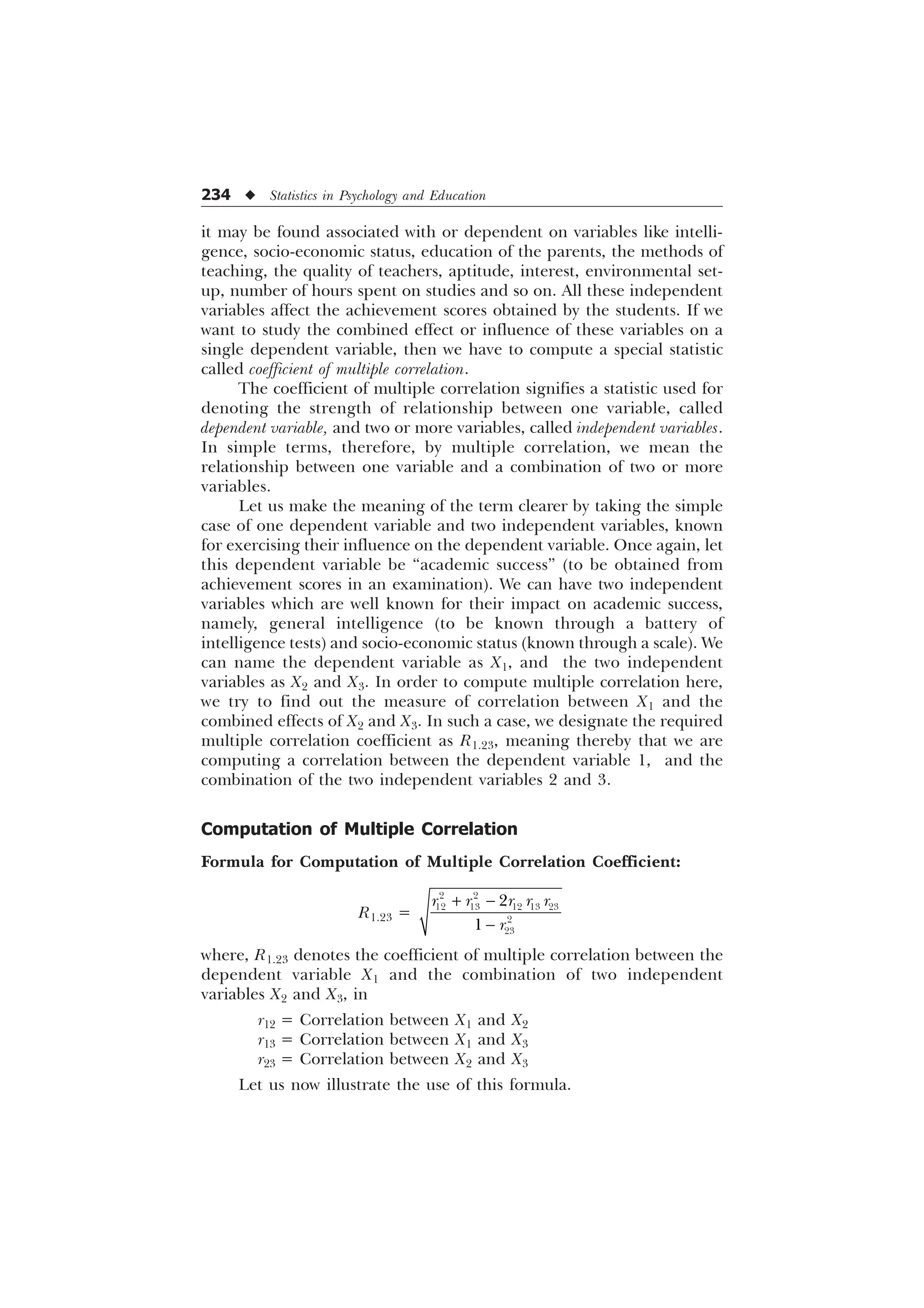
NEED AND IMPORTANCE OF MULTIPLE CORRELATION
In many studies related to education and psychology, we find that a
variable is dependent on a number of other variables called independent
variables. For example, if we take the case of one’s academic achievement,](https://image.slidesharecdn.com/stats-s-241206101830-e3d4cc67/75/Stats-S-K-Mangal-statistics-textook-in-pdf-245-2048.jpg)
![Partial and Multiple Correlation u 235
Example 13.3: In a study, a researcher wanted to know the impact of
a person’s intelligence and his socio-economic status on his academic
success. For computing the coefficient of multiple correlation, he
collected the required data and computed the following inter-
correlations:
r12 = 0.60, r13 = 0.40, r23 = 0.50
where 1, 2, 3 represent the variables “academic success”, “intelligence”
and “socio-economic status”, respectively. In this case, find out the
required multiple correlation coefficient.
Solution. The multiple correlation coefficient
R1.23 =
¹ ¹
U U U U U
U
Substituting the respective values of r12, r13 and r23 in the above formula,
we get
R1.23 =
– – –
=
[Ans. Multiple correlation coefficient = 0.61.]
Other Methods of Computing Coefficient of Multiple
Correlation
Multiple correlation coefficient can also be computed by other means
like below.
First, it can be done with the help of partial correlation. Thus,
R1.23 =
U U
In this formula, to understand the relationship between variable 1 and
the combined effect of variables 2 and 3, we compute the multiple
correlation coefficient. The formula requires the values of r12
(correlation between 1 and 2) and the partial correlation r13.2, which can
be computed by using the formula
r13.2 =
U U U
U U
However, in case if there are four variables instead of three, then
we can compute the multiple correlation coefficient as](https://image.slidesharecdn.com/stats-s-241206101830-e3d4cc67/75/Stats-S-K-Mangal-statistics-textook-in-pdf-247-2048.jpg)
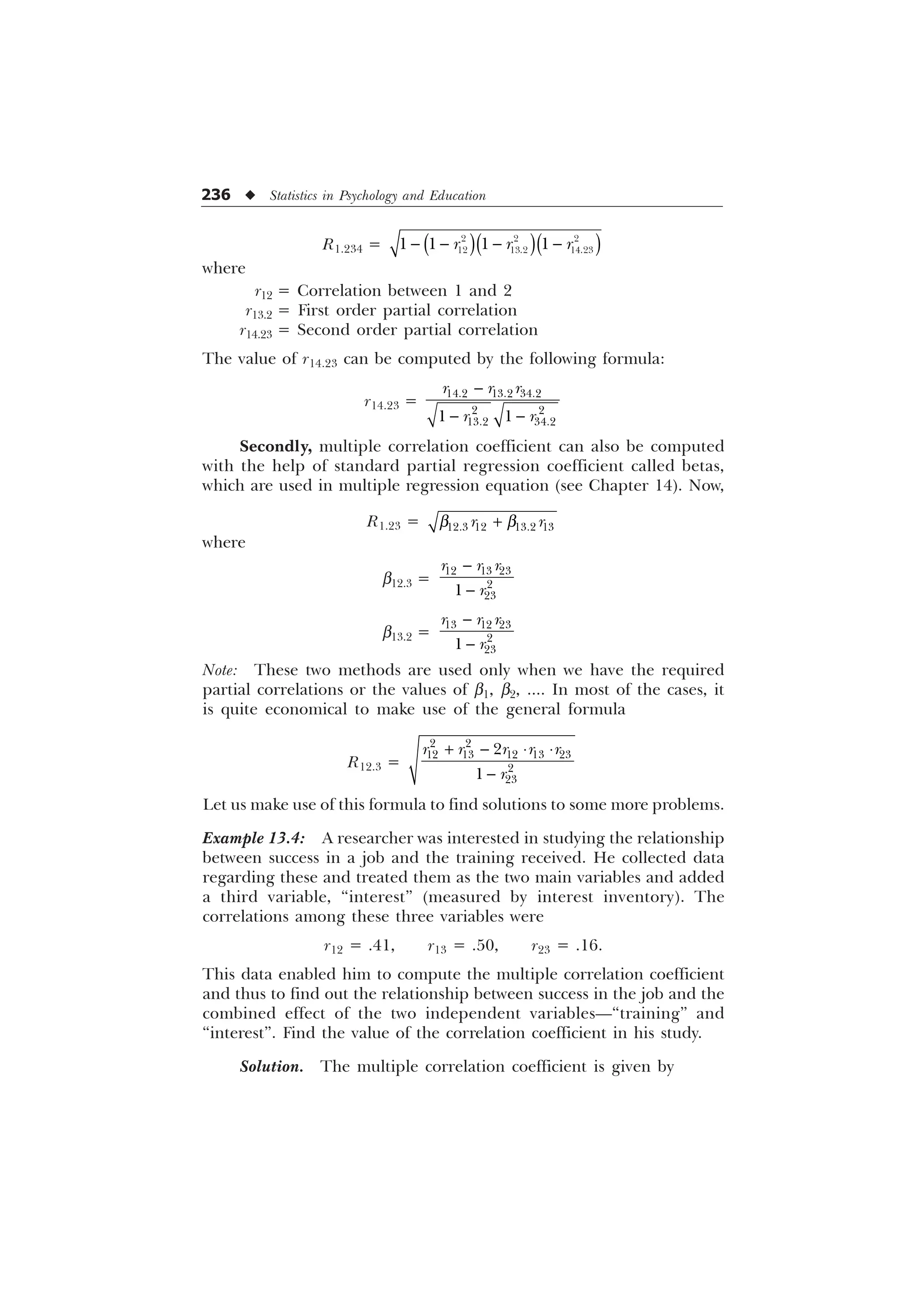
![Partial and Multiple Correlation u 237
R1.23 =
U U U U U
U
=
– – –
=
=
= 0.601
[Ans. Multiple correlation coefficient = 0.601.]
Example 13.5: One thousand candidates appeared for an entrance test.
The test had some sub-tests, namely, general intelligence test,
professional awareness test, general knowledge test and aptitude test. A
researcher got interested in knowing the impact or the strength of the
association of any two sub-tests on the total entrance test scores (X1).
Initially, he took two sub-tests scores—intelligence test scores (X2) and
professional awareness scores (X3)—and derived the necessary
correlations. Compute the multiple correlation coefficient for
measuring the strength of relationship between X1 and (X2 + X3), if
r12 = .80, r13 = .70 and r23 = .60.
Solution. The multiple correlation coefficient
R1.23 =
U U U U U
U
=
– – –
=
=
= 0.845
[Ans. Multiple correlation coefficient = 0.845.]](https://image.slidesharecdn.com/stats-s-241206101830-e3d4cc67/75/Stats-S-K-Mangal-statistics-textook-in-pdf-249-2048.jpg)